A computational model of stereoscopic prey capture in praying mantises

Abstract

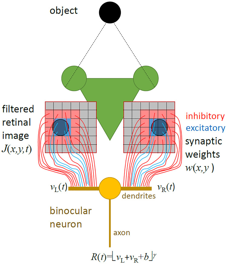
We present a simple model which can account for the stereoscopic sensitivity of praying mantis predatory strikes. The model consists of a single "disparity sensor": a binocular neuron sensitive to stereoscopic disparity and thus to distance from the animal. The model is based closely on the known behavioural and neurophysiological properties of mantis stereopsis. The monocular inputs to the neuron reflect temporal change and are insensitive to contrast sign, making the sensor insensitive to interocular correlation. The monocular receptive fields have a excitatory centre and inhibitory surround, making them tuned to size. The disparity sensor combines inputs from the two eyes linearly, applies a threshold and then an exponent output nonlinearity. The activity of the sensor represents the model mantis's instantaneous probability of striking. We integrate this over the stimulus duration to obtain the expected number of strikes in response to moving targets with different stereoscopic disparity, size and vertical disparity. We optimised the parameters of the model so as to bring its predictions into agreement with our empirical data on mean strike rate as a function of stimulus size and disparity. The model proves capable of reproducing the relatively broad tuning to size and narrow tuning to stereoscopic disparity seen in mantis striking behaviour. Although the model has only a single centre-surround receptive field in each eye, it displays qualitatively the same interaction between size and disparity as we observed in real mantids: the preferred size increases as simulated prey distance increases beyond the preferred distance. We show that this occurs because of a stereoscopic "false match" between the leading edge of the stimulus in one eye and its trailing edge in the other; further work will be required to find whether such false matches occur in real mantises. Importantly, the model also displays realistic responses to stimuli with vertical disparity and to pairs of identical stimuli offering a "ghost match", despite not being fitted to these data. This is the first image-computable model of insect stereopsis, and reproduces key features of both neurophysiology and striking behaviour.

Fig 1. Praying mantis viewing a simulated target in (A) crossed and (B) uncrossed geometry.

Each element of the target is displayed on a screen 10 cm away, well outside the catch range. Coloured filters placed over the mantid’s eyes ensure that each eye sees only the intended target. In (A), the target is simulated as being at 2.5 cm, where the lines of sight cross, eliciting a strike. In (B), left and right images are exchanged so the lines of sight diverge. mantids rarely strike at such stimuli [10, 11].

Fig 2. Schematic diagram of the disparity energy model.

The model postulates a binocular neuron which receives input from each eye, representing the inner product of the retinal image with a receptive field function. The receptive field function represents the effect of stimulation at each point in the retinal image on the binocular neuron, and can be thought of as an effective synaptic weight (though the real pathway is multisynaptic). Red and blue are used to represent inhibitory and excitatory weights respectively. The activity of the neuron is then represented as a nonlinear function of its total input. In the original energy model [24], this nonlinearity was a threshold at 0 followed by squaring; we generalise the model to allow for a non-zero threshold −b and arbitrary exponent γ. Mathematical symbols are defined below, Eqs (1) and (2). We postulate that this binocular neuron synapses onto a motoneuron in such a way that the instantaneous strike probability is proportional to the activity of the binocular neuron.

Fig 3. Response of real neuron (A, columnar commissural neuron rr160127 from [22]), along with response (C) predicted by the disparity energy model with the receptive field functions shown in B,D for left, right eyes.

Here, due to experimental constraints on recording time, the stimuli were long vertical bars 13° in width, so the receptive fields are obtained only coarsely and as a function of only horizontal position. The receptive fields in both eyes have an excitatory centre (positive weights, blue) and inhibitory surround (negative, red). In the receptive fields fitted to this particular neuron, the excitatory centre is wider in the left eye than the right eye; elsewhere in this paper, we enforced symmetry for simplicity. The fitted threshold here is b = 0 and the output exponent is γ = 2.24; see Eqs (1) and (2). See [22] and its Supplementary Information for a detailed description of how responses are plotted in A and C for the real and model neuron respectively. Briefly, the marginal plots show the responses to monocular bars flashed in left or right eyes. The pseudocolor shows the responses to binocular bars, with the location in left, right eyes given by the location along vertical, horizontal axes. The olive lines mark the azimuthal location of the stimulus and the gray lines its disparity (dashed line indicates infinite simulated distance, or zero disparity). This neuron responded best to a bar flashed at a location corresponding to 2.5cm away on the midline.

Fig 4. Sensitivity of mantis striking behaviour to stimulus size and stereoscopic distance.

(A) Data from [10], available at http://dx.doi.org/10.1098/rstb.2015.0262. Species was Sphodromantis lineola; stimuli were on a computer screen 10cm from the insect; nearer distances were simulated using coloured filters. (B) Data extracted from Fig 5 of [36] using WebPlotDigitiser (https://apps.automeris.io/wpd/). Species was Sphodromantis viridis; stimuli were on a computer screen 5.5cm from the insect; nearer distances were simulated using base-out prisms. Note that in this figure, we plot the strike rate, i.e. the probability that a given trial elicits striking behaviour (since this was what was available for [36]). In [10], some trials elicited several strikes. The peak strike rate in A, 0.49, is lower than the peak of the mean number of strikes, plotted below in Fig 9.

Fig 5. Spatiotemporal filtering, for a disk of diameter 11° moving from left to right.

A: Pattern of light incident on the retina at a particular moment of time. B: After spatial filtering through a Gaussian with a standard deviation of 0.7°, representing the acceptance angle of foveal mantis ommatidia. C: The resulting neural input, after temporal filtering and squaring. There is activity only at the leading and trailing edges of the disk, where the retinal stimulus is changing.

Fig 6. The image shows left- and right-eye receptive fields, superimposed and backprojected onto a screen at 10cm distance for ease of comparison with the stimuli.

The left- and right-eye receptive fields have identical structures, with a central strongly excitatory region (blue) surrounded by an outer, more weakly excitatory region (purple), and then by a much larger inhibitory region (pink). The receptive fields in the two eyes appear offset horizontally on the screen by the screen disparity d = 15.4°.

Fig 7. Variance versus mean for number of strikes per trial.

Symbols labeled “2016-crossed/uncrossed” represent data from [10]; GM-A-D are from our ghost-match experiments, see Fig 10 below. We pooled data from all trials in all mantids for a given stimulus (disk size and geometry), and computed the mean and variance of the number of strikes observed across trials. The number of trials contributing to each data-point is 68 for the data from [10], 120 for the GM-D condition and 170 for GM-A,B,C. Symbols encode disk diameter in degrees; color encodes stimulus geometry and data-set. The scatterplot shows variance plotted against mean, with the black line marking the identity. For a Poisson distribution, variance = mean and so points should lie on the identity.

Fig 8. Top-down view (not to scale) of a mantis viewing a computer screen at a distance S.

To simulate an object at distance D from the mantis, the left and right eye’s images (labelled L, R) need to be separated by a distance P on the screen. The angle subtended by the distance P at the mantis is the screen disparity α; the retinal disparity Δ of the virtual object is the angle subtended by the interocular distance I at the virtual object.

Fig 9. Modified behavioural response of mantids.

Mean number of strikes [10] in response to different simulated distances, as a function of the angular size of the simulated target in the crossed condition, with strikes in the corresponding uncrossed condition subtracted. Ribbons show ±1 standard error on the mean.

Fig 10. Testing the response of model and mantids to ghost matches.

Top row shows four different stimulus geometries: (A) a single object 2.5cm distant from the mantis, simulated by disparate objects on a screen 10cm distant, with screen parallax 2.1cm; (B) two objects 10cm distant, 2.1cm apart; (C) as A but with an additional image presented to each eye, with diverging lines of sight meaning that these cannot correspond to any one physical object; (D) single object 10cm distant. Middle row indicates how each of these appear on the screen as viewed by the right and left eye, for the two different disk diameters used. Bottom row: Mean number of strikes elicited per trial for each size and stimulus geometry. Coloured lines: average over 10 trials for each of 18 mantids (not all mantids were tested on the control condition D). Black dots: group average over all mantids; errorbars, ± standard error. Red symbols: mean number of strikes predicted by the model, for horizontal motion (⊳), vertical motion (▽), and for the average of the two (◊).

Fig 11. Mean number of strikes per trial predicted by the fitted model, as a function of stimulus size (horizontal axes) and simulated distance (colours).

The top row is for targets moving horizontally over the sensor; the middle for stimuli moving vertically, and the bottom row for the average of both. The left panels are for crossed stimuli and the right for uncrossed. In all cases, the target passed directly over the receptive field center. The dashed lines in the crossed panels show the empirical data from [10] (Table 3) which the optimisation aimed to reproduce. In the experiments, the target had a spiralling motion with both horizontal and vertical components, so the same empirical data are shown in all three rows. As described in the Methods (see Table 3), the optimisation also aimed to predict zero strikes for stimuli at 10cm simulated distance, for monocular stimuli, and for stimuli of size 38° diameter. The other conditions—intermediate sizes and disparities, and uncrossed stimuli—were not constrained in the fitting, but the model structure ensures that plausible results are also obtained for these.

Fig 12. Responses of different model components to a horizontally-moving disk at a simulated distance of 2.5cm from the mantis.

Left, middle, right columns are for a target of size 11.2°, 16.9° and 25.5° as indicated. Sub-panels in the top two rows show left and right eyes. In all panels, axis coordinates are in degrees visual angle referred to the centre of the screen, i.e. x = 0, y = 0 corresponds to a location 10cm directly in front of the mantis. However, the interpretation of the axes differs in each row, as explained below. Top row (ABC): Snapshots of the filtered images J_L,R(x, y, t), shown as a function of retinal location (x, y) for one particular time t. The axes are therefore simply retinal location. Pseudocolor represents the images reaching the sensor’s receptive fields, following lowpass spatial filtering, highpass temporal filtering and squaring in the early visual system. The receptive field excitatory region is shown superimposed for comparison. Each pixel represents the value of the filtered image at a particular location in the retina. These snapshots are for one particular time t and thus for one particular target position x_tgt(t), y_tgt(t) as the target moves across the screen. In this figure, the target was moving horizontally, so y_tgt is in fact independent of time whereas x_tgt = x₀ + Vt. The yellow circle marks where the center of the target is in that eye at the time shown. The white cross marks the center of the sensor receptive field in that eye; the inner white square marks the boundary of the central excitatory region, while the outer white square marks the boundary of the outer excitatory region. The surrounding inhibitory region extends beyond the range shown in each panel. Thus, parts of the filtered image falling outside the white squares have an inhibitory effect on the sensor. Middle row (DEF): Inputs to the binocular disparity sensor from the two eyes, v_L,R. The input from each eye is the inner product of the monocular receptive field with the filtered image at that moment in time. It is here represented as a function of target position x_tgt(t), y_tgt. Since the target is moving horizontally across the screen from left to right, x_tgt is a function of time, whereas y_tgt is constant for a given trajectory. Each pixel-row in DEF therefore represents the time-course of the monocular input, v_L,R(t), as the target moves from left to right over the screen, at the vertical location y_tgt corresponding to the height of the pixel row. The axes therefore represent the current location of the target in the retina, and the panel as a whole does not represent an image, since different locations correspond to different times. The pink arrows mark the value of the monocular input in D for the filtered image shown in A. Bottom row (GHI): response of the disparity sensor, Eq 2. The axes are now the current visual direction of the moving binocular target, x_c(t) = 0.5(x_tgtL(t) + x_tgtR(t)); x_c is again a function of time. Arrows from D to G show the target locations shown in the top row, A, and thus the response when the target crosses the midline, x_c = 0. For comparison, dotted arrows show the response a little earlier when x_c was −6°. The target’s direction in the visual field is x_c = (x_tgtL + x_tgtR)/2 and y_c = (y_tgtL + y_tgtR)/2. Since the target is moving horizontally, x_c is a function of time, but y_c is constant for a given trajectory.

Fig 13. Model sensor output R(x_c, y_c) for horizontally or vertically travelling targets as they move across the centre of the field of view.

Different rows are for different target distances, as indicated down the left-hand side of the figure, while different target sizes are in columns, as indicated along the bottom. The pseudocolour shows the instantaneous response of the disparity sensor as the centre of the moving target first reaches the location indicated by the (x,y) position. (To simulate the 60Hz refresh rate of the monitor, the target changes position every 16ms, and so stays in each location for five of the simulation’s 3.3ms timesteps). The color axis is the same in all 24 panels.

Fig 14. As for Fig 12, but for a target at a simulated distance of 10cm from the mantis (zero screen disparity).

Fig 15. Predicted strike rate M_model (Eq 3) for disks moving horizontally (A-L) or vertically (M-X) in front of the model mantis, as a function of vertical disparity Δy and offset perpendicular to the direction of motion (y_c for horizontally-moving targets and x_c for vertically-moving).

For the horizontally-moving targets, the vertical location of the target in the two eyes is constant at y_L = y_c + Δy/2 and y_R = y_c − Δy/2. For vertically-moving targets, the mean y-location is of course a function of time, but the difference y_L − y_R is constant at Δy. Different rows are for different disparities, thus simulating disks at different distances from the animal when Δy = 0. Different columns are for different disk diameters.

Fig 16. Sensitivity to vertical disparity and size, for our model (solid lines) and empirical data digitized from [31].

A: Solid lines show strike rate predicted by our model, averaged across horizontally and vertically travelling targets passing directly over the sensor. Dashed lines show strike rates observed by [31] for stationary “jiggling” targets. Colors indicate target size as shown in the legend. B: as A but the strike rate is normalized to be 1 for stimuli with zero vertical disparity.

References

1. Nityananda V, Read JCA. Stereopsis in animals: evolution, function and mechanisms. Journal of Experimental Biology. 2017;220(14):2502–2512. doi: 10.1242/jeb.143883 - DOI - PMC - PubMed
1. Read JCA. Binocular vision and stereopsis across the animal kingdom. Annual Review of Vision Science. 2021;. doi: 10.1146/annurev-vision-093019-113212 - DOI - PubMed
1. Gonzalez-Bellido PT, Talley J, Buschbeck EK. Evolution of visual system specialization in predatory arthropods. Current Opinion in Insect Science. 2022; p. 100914. doi: 10.1016/j.cois.2022.100914 - DOI - PubMed
1. Ambrosch K, Kubinger W. Accurate hardware-based stereo vision. Computer Vision and Image Understanding. 2010;114(11):1303–1316. doi: 10.1016/j.cviu.2010.07.008 - DOI
1. Humenberger M, Zinner C, Weber M, Kubinger W, Vincze M. A fast stereo matching algorithm suitable for embedded real-time systems. Computer Vision and Image Understanding. 2010;114(11):1180–1202. doi: 10.1016/j.cviu.2010.03.012 - DOI
Publication types