Emergent reliability in sensory cortical coding and inter-area communication

Abstract

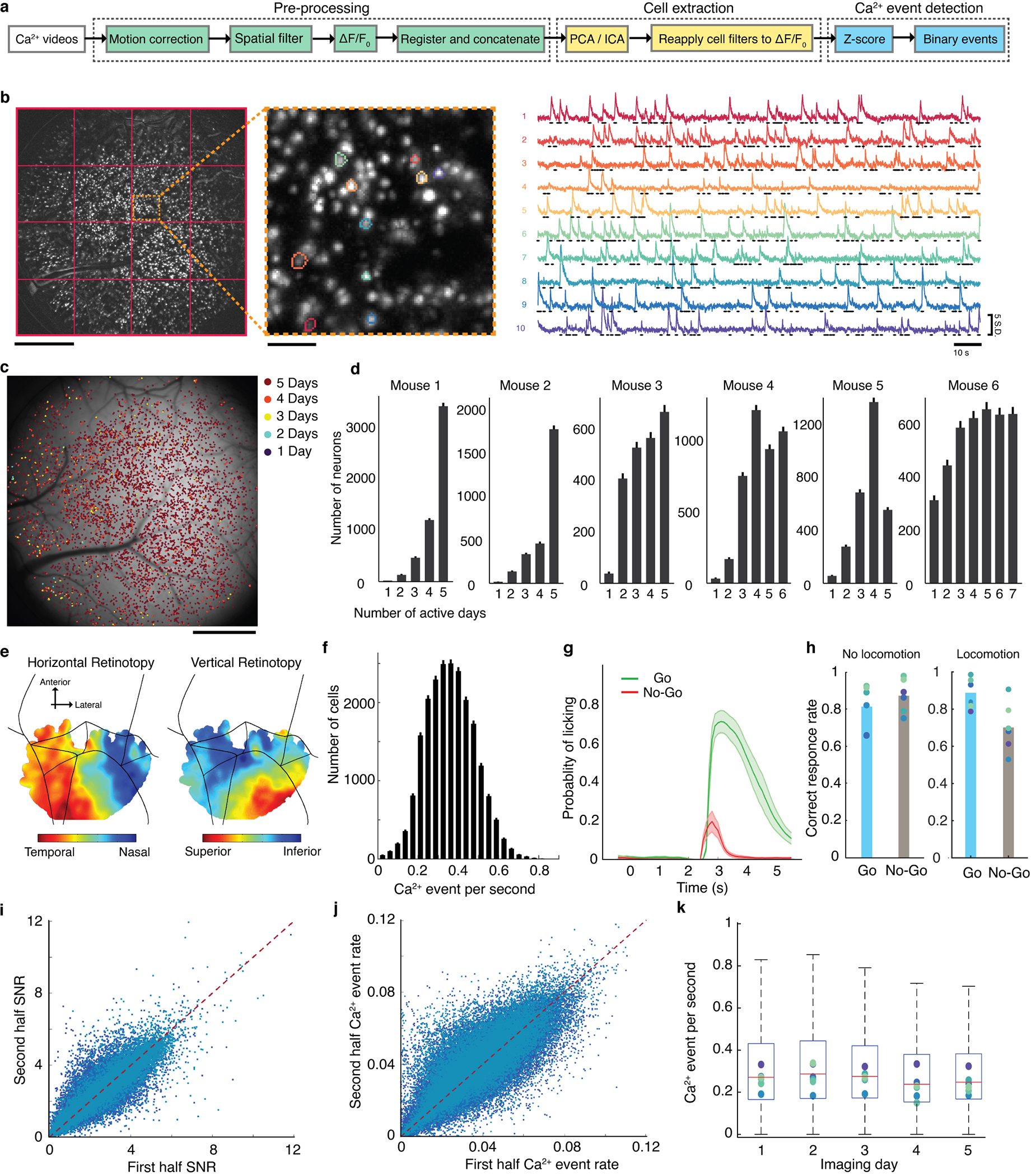
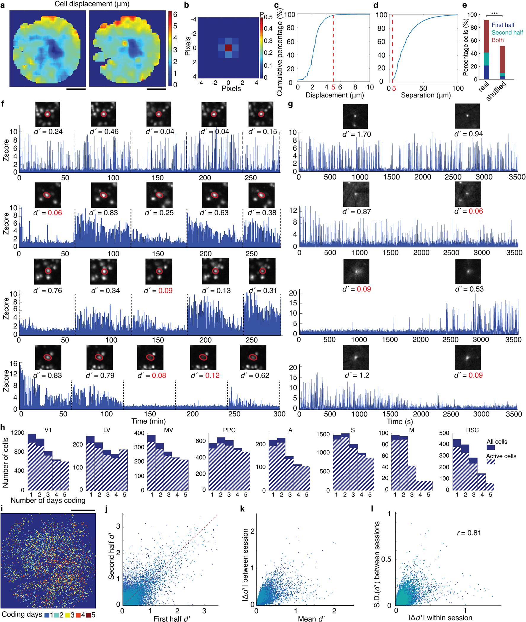
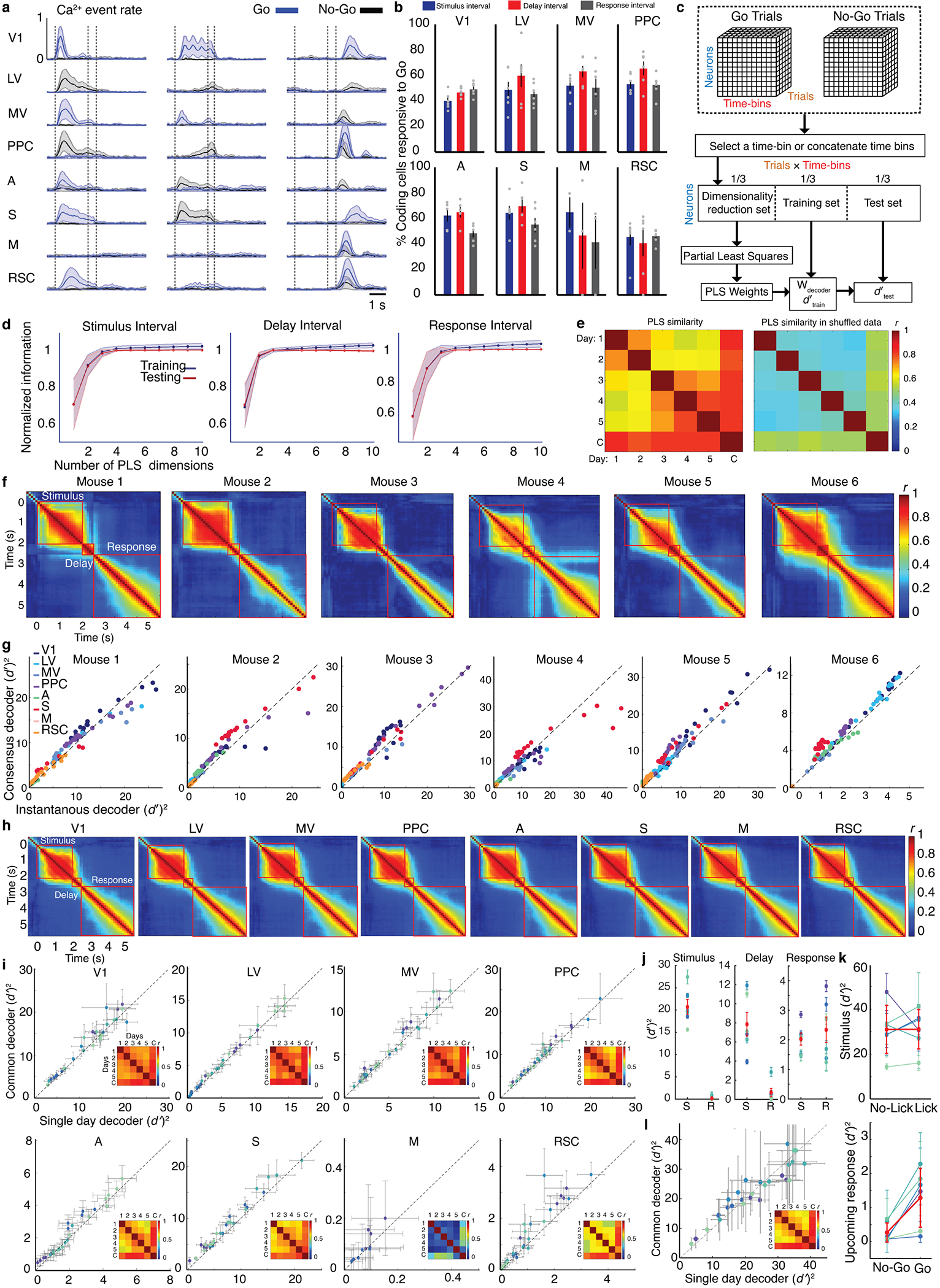
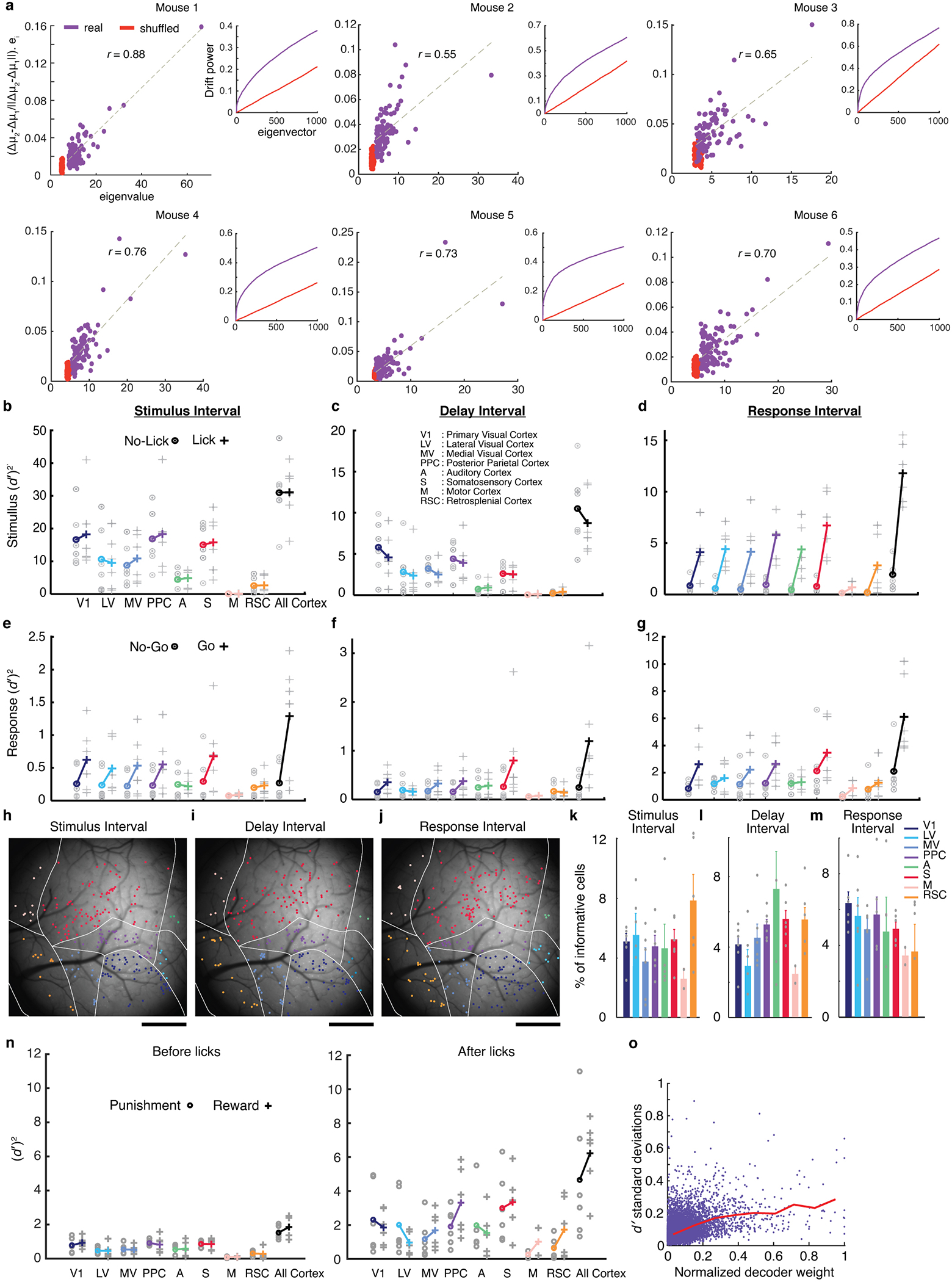
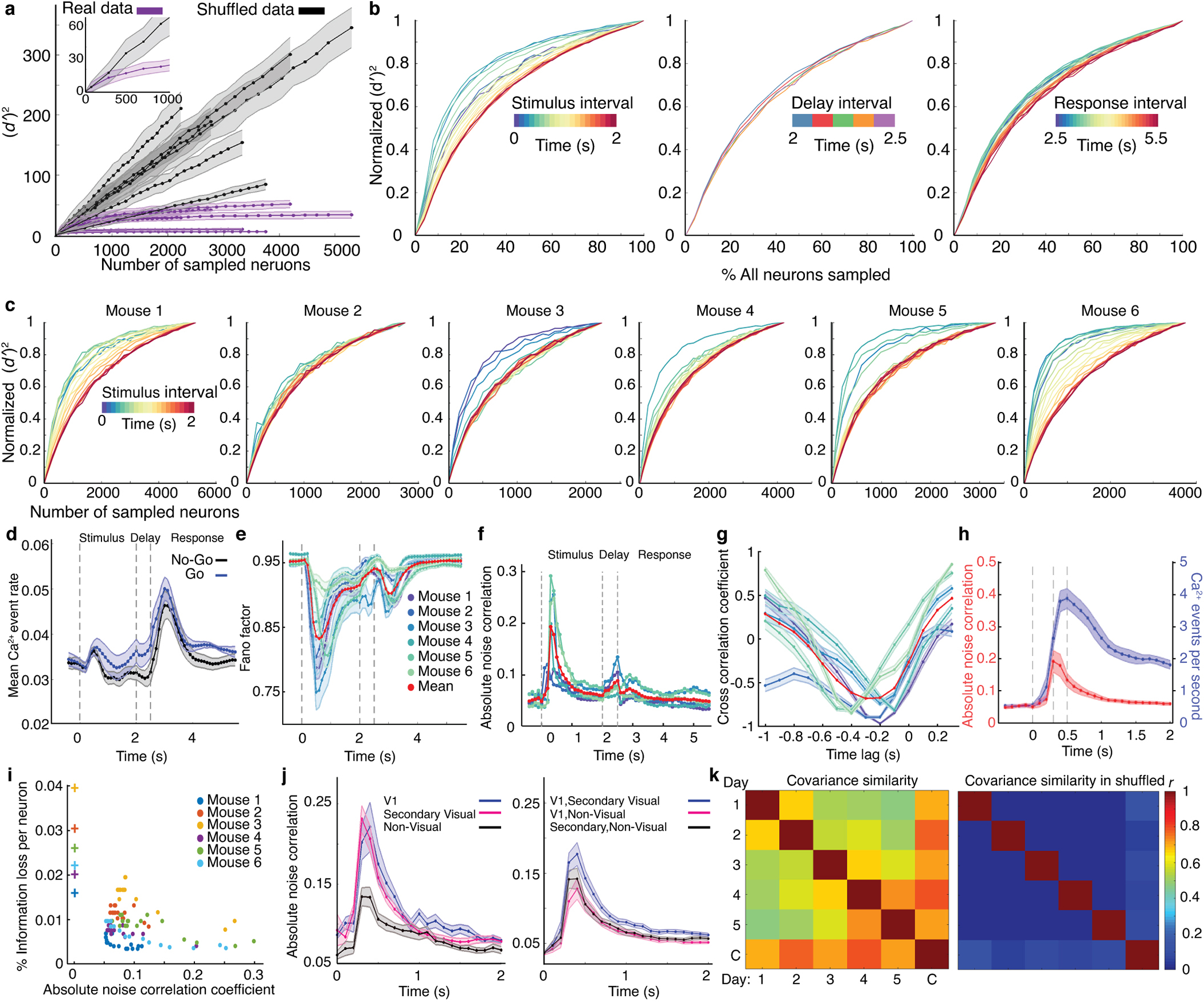
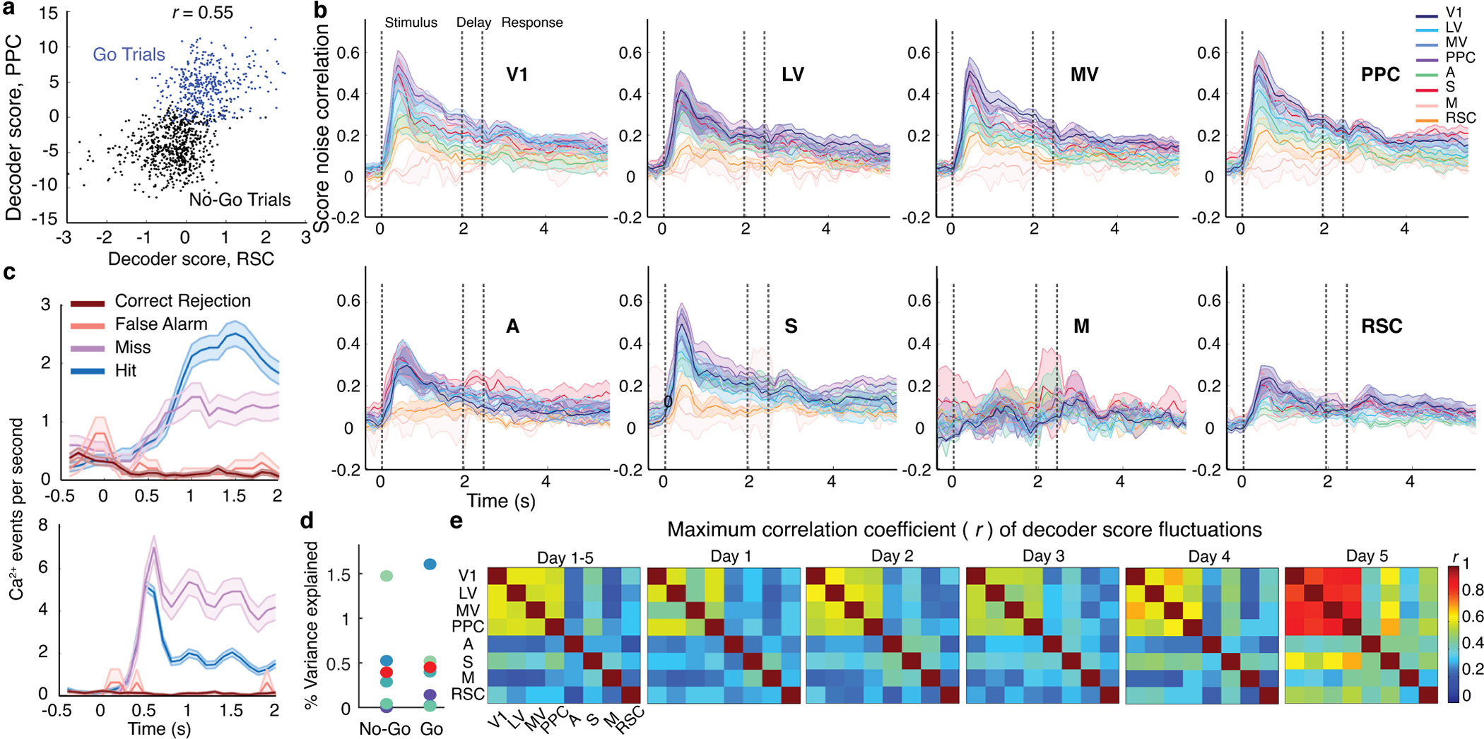
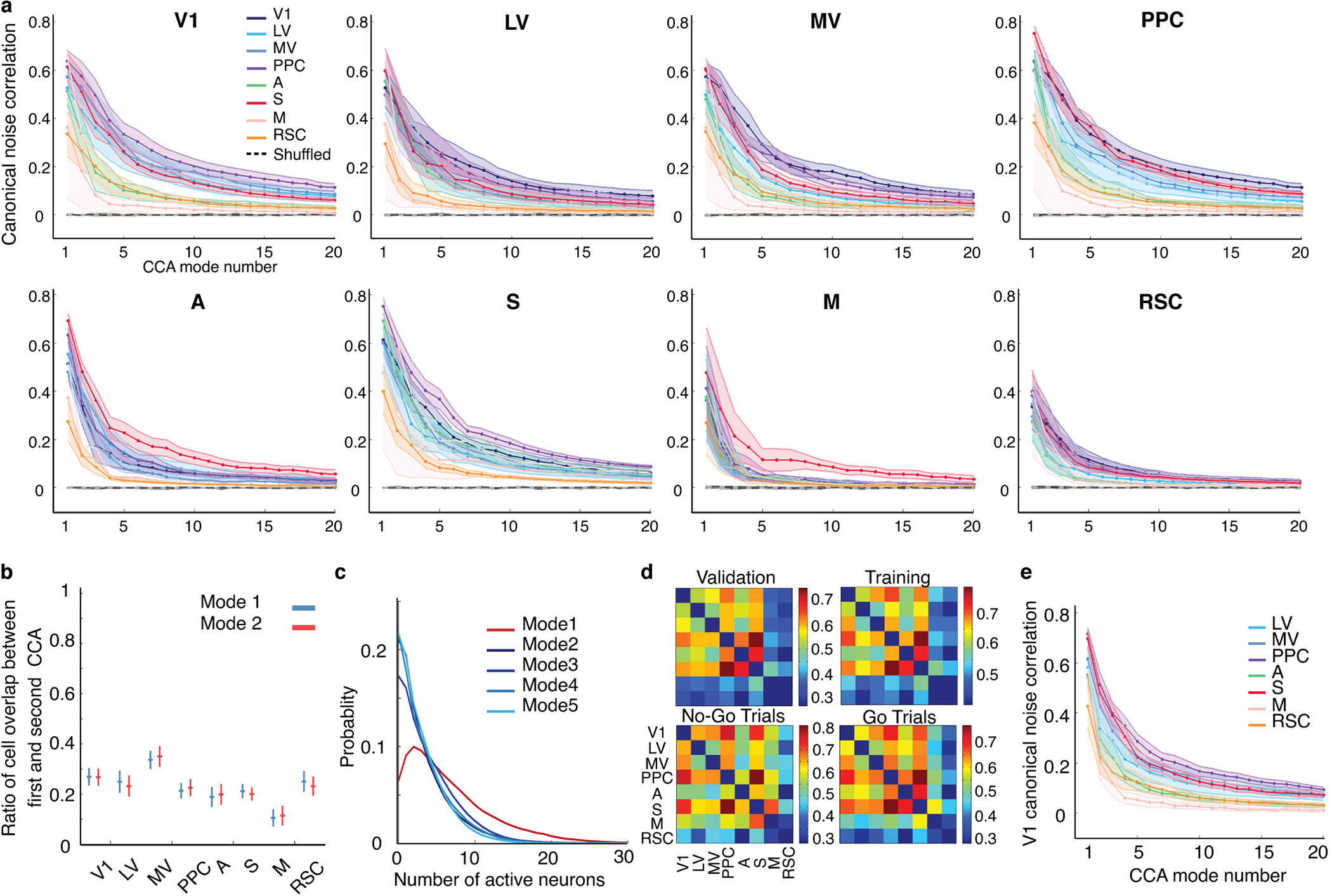
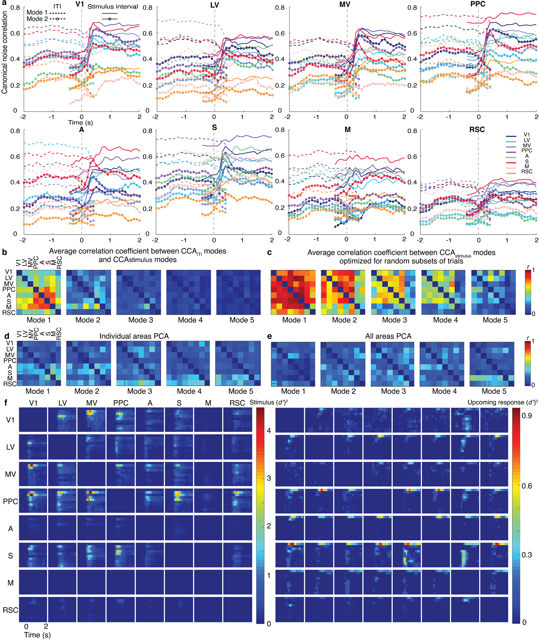
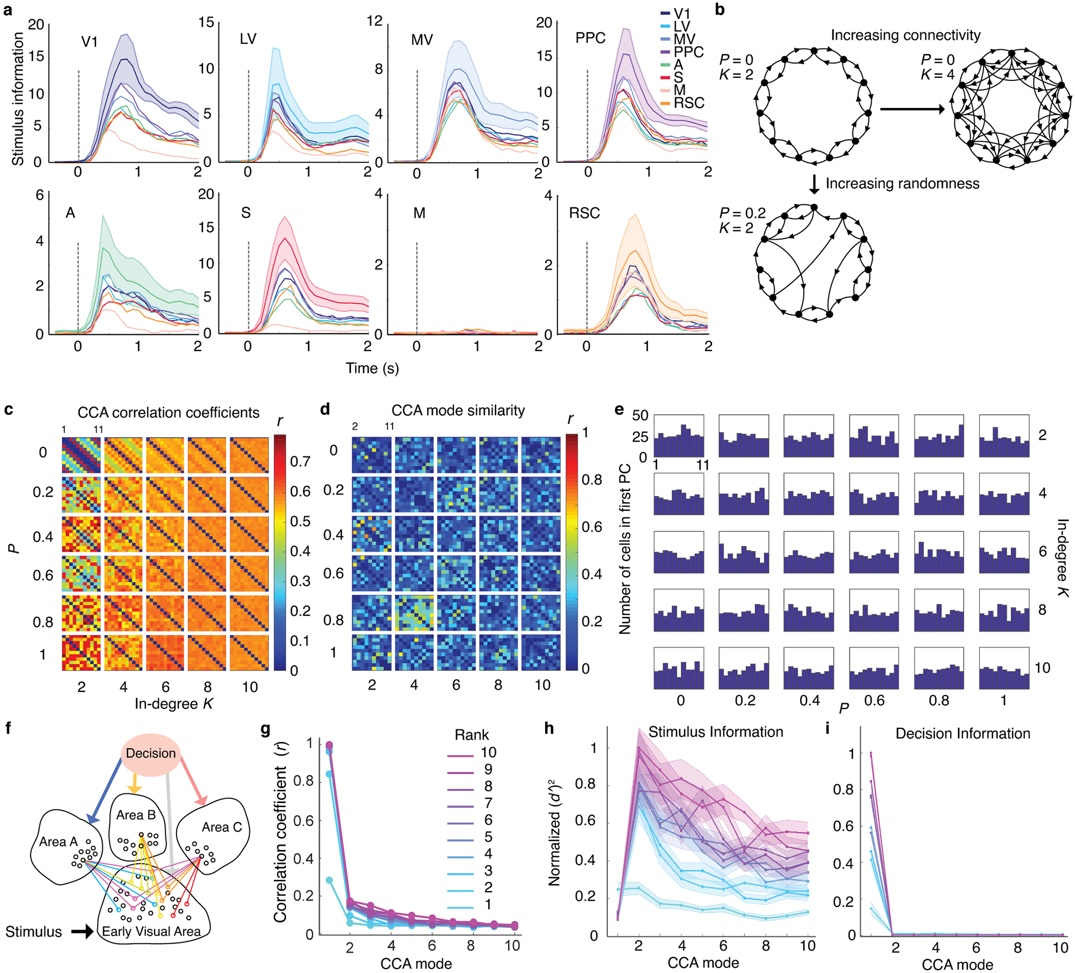
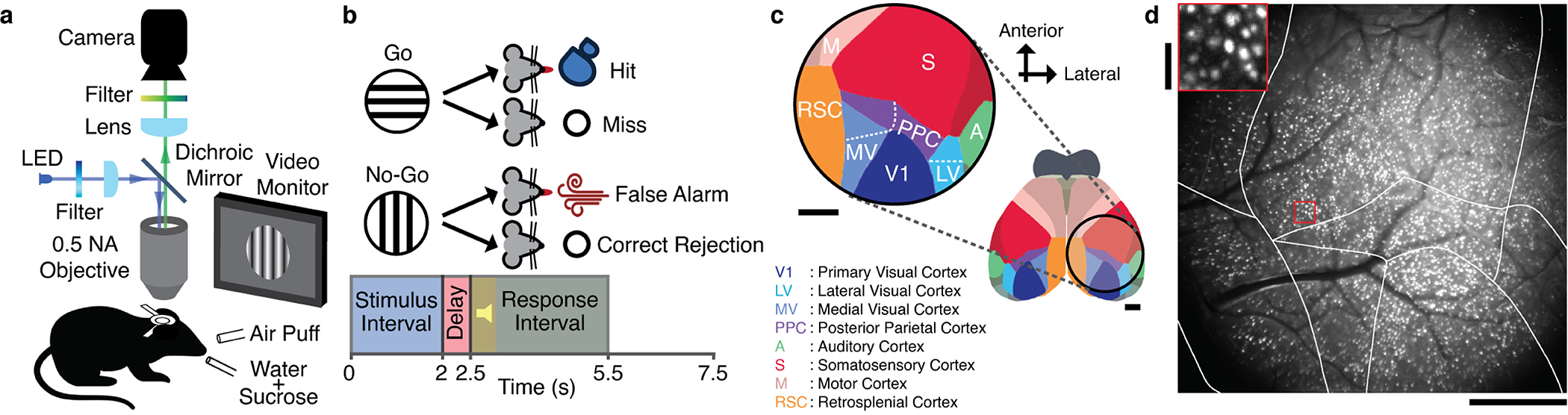
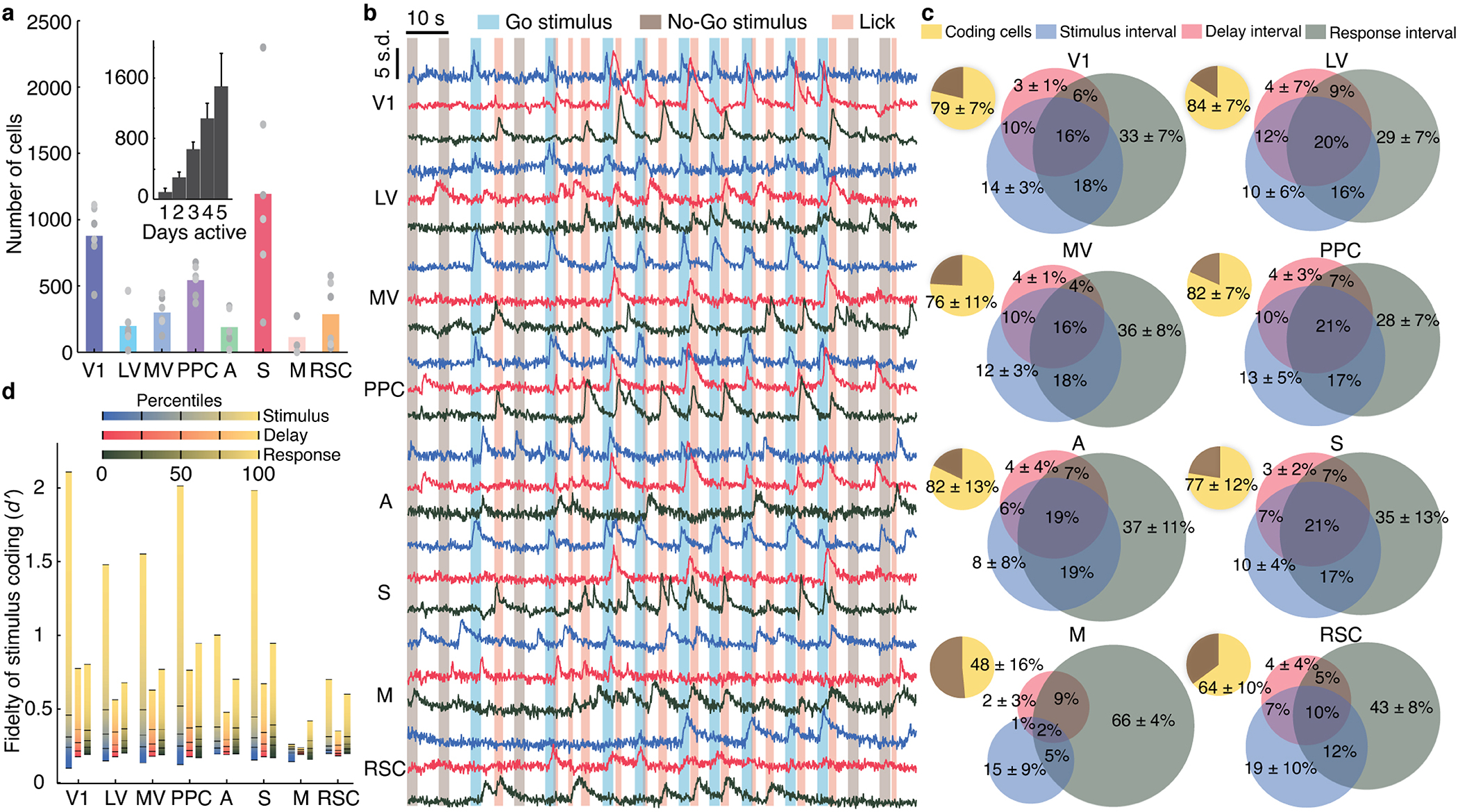
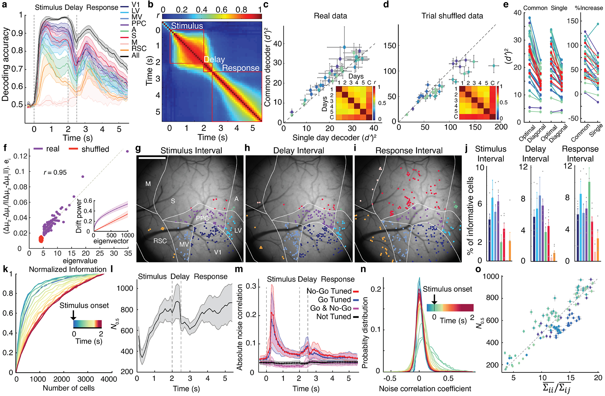
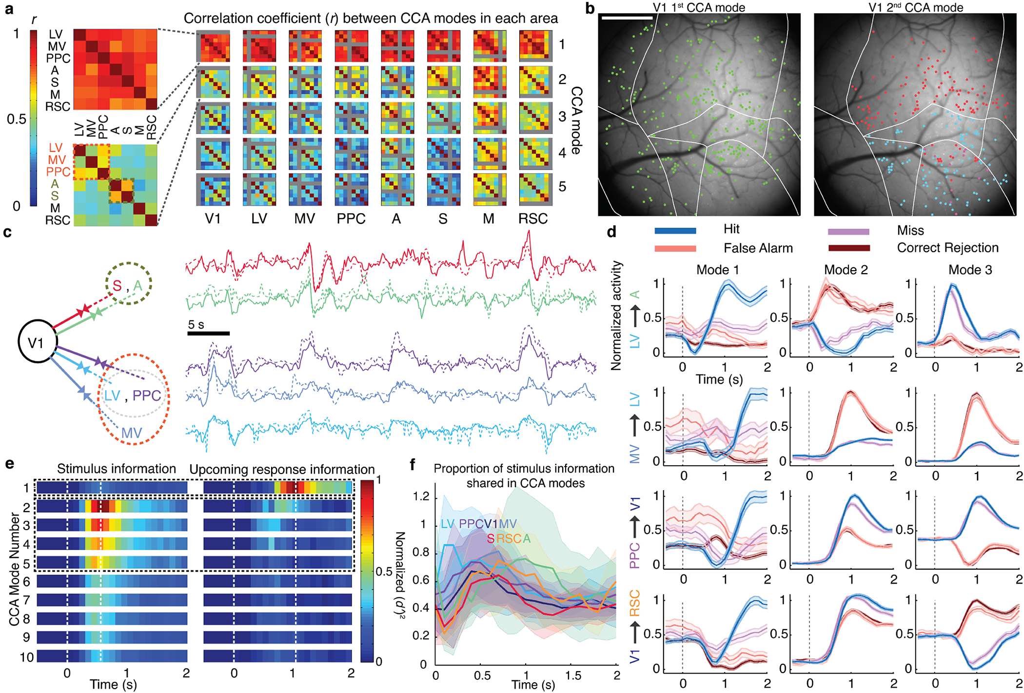
Reliable sensory discrimination must arise from high-fidelity neural representations and communication between brain areas. However, how neocortical sensory processing overcomes the substantial variability of neuronal sensory responses remains undetermined^1-6. Here we imaged neuronal activity in eight neocortical areas concurrently and over five days in mice performing a visual discrimination task, yielding longitudinal recordings of more than 21,000 neurons. Analyses revealed a sequence of events across the neocortex starting from a resting state, to early stages of perception, and through the formation of a task response. At rest, the neocortex had one pattern of functional connections, identified through sets of areas that shared activity cofluctuations^7,8. Within about 200 ms after the onset of the sensory stimulus, such connections rearranged, with different areas sharing cofluctuations and task-related information. During this short-lived state (approximately 300 ms duration), both inter-area sensory data transmission and the redundancy of sensory encoding peaked, reflecting a transient increase in correlated fluctuations among task-related neurons. By around 0.5 s after stimulus onset, the visual representation reached a more stable form, the structure of which was robust to the prominent, day-to-day variations in the responses of individual cells. About 1 s into stimulus presentation, a global fluctuation mode conveyed the upcoming response of the mouse to every area examined and was orthogonal to modes carrying sensory data. Overall, the neocortex supports sensory performance through brief elevations in sensory coding redundancy near the start of perception, neural population codes that are robust to cellular variability, and widespread inter-area fluctuation modes that transmit sensory data and task responses in non-interfering channels.

Extended Data Fig. 1.. Long-term imaging and computational analysis of neural Ca²⁺ dynamics across multiple cortical areas during a visual discrimination task.

(a) Schematic of the algorithmic pipeline used for video preprocessing and cell extraction, as implemented using cluster computing. Pre-processing (steps shown in green): For each movie of Ca²⁺ activity, we performed an image registration across all frames of the movie to correct for small displacements of the brain. We removed background noise and neuropil Ca²⁺ activity by applying a spatial Gaussian high-pass filter $(\sigma =80\mu \mathrm{m})$, and computed a movie of the relative changes in fluorescence $\left(\mathrm{\Delta }F\left(t\right)/F_0\right)$. We then aligned and concatenated all the $\mathrm{\Delta }F\left(t\right)/F_0$) movies for each individual mouse, across all imaging sessions. Cell extraction (steps shown in yellow): We divided each concatenated movie into 16 spatial tiles and then extracted individual cells within each tile by successively applying principal components and independent components analyses (PCA/ICA algorithm) to all tiles in parallel using the Stanford Sherlock computing cluster (using up to 320 cores and ~2 TB of memory for each concatenated movie). Ca²⁺ event detection (steps shown in cyan): We converted the $\mathrm{\Delta }F\left(t\right)/F_0$) traces for each neuron to traces expressing the time-dependent fluorescence changes as a z-score, $z\left(t\right)$, relative to the s.d. of the baseline fluctuations in each cell’s fluorescence trace (computed separately for each imaging session). We detected Ca²⁺ events by identifying Ca²⁺ transients that attained a peak fluorescence value of $z\left(\mathrm{t}\right)\ge 4$ s.d., and we assigned the cell as being ‘active’ within the interval between the initial threshold crossing and the time at which the Ca²⁺ event attained its peak fluorescence (Methods). (b) Left: A maximum projection image over an entire concatenated set of Ca²⁺ movies from an example mouse. Red lines mark the 4 × 4 set of tiles that we processed in parallel during cell extraction. Scale bar: 1 mm. Middle: Magnified view of the area enclosed in orange in the left panel. Scale bar: 0.1 mm. Right: Z-scored traces (colored traces) of fluorescence Ca²⁺ activity for 10 example neurons in the middle panel marked with color-corresponding boundaries. Raster traces show the binarized patterns of activity for each cell. (c) Most detected cells were active in all recording sessions, as illustrated via a map, computed for one example mouse, in which each detected cell is marked with a color-code indicating the number of days in which it was detected as active (Methods). (d) Histograms of the number of days that each cell was detected as active for 6 different mice. Error bars are s.d. estimated as counting errors. (e) Vertical and horizontal retinotopic maps of visual cortex in an example mouse (Methods). After identifying borders of area V1 determined by retinotopic mapping studies in each mouse, we aligned these borders with those in the Allen Brain Observatory map of the mouse cortex and thereby inferred the locations of other brain areas. (f) Histogram of the mean Ca²⁺ event rate for each of 21,570 cortical neurons (N = 6 mice). Error bars are s.d. estimated as counting errors. (g) Mean probability of licking over the time course of a trial, averaged over all trials and trained mice, for Go (green) and No-Go (red) trials. Shaded areas denote s.e.m. over N = 6 mice. After mice learned to discriminate between Go and No-Go visual stimuli, we trained them to withhold licking behavior during the stimulus presentation, [0 s, 2 s], and delay, [2 s, 2.5 s], intervals and to respond only during the response interval, [2.5 s, 5.5 s] (Fig. 1; Methods). Trained mice occasionally licked before the response interval; we discarded these trials from our analyses to allow inferences regarding stimulus encoding, decision-making, and motor preparation in the absence of overt licking responses. (h) The mean behavioral performance of all mice on Go (cyan) and No-Go (gray) trials in which the mouse did (right) or did not exhibit locomotor behavior (left) (Methods). Individual data points denote values from individual mice. (i, j) For every individual cell (blue data points), the plots show the mean signal-to-noise ratio (SNR) of Ca²⁺ activity, i, or the mean rate of Ca²⁺ transient events, j, in the first half of each imaging session versus that in the second half of the same session. From linear regression, the mean SNR and Ca²⁺ event rate in the second half of each session were 96 ± 2 % (N = 6 mice) and 99 ± 3 % (N = 6 mice), respectively, of their values in the first half. (k) A box and whisker plot of the Ca²⁺ event rate across all cells imaged for 5 days in each mouse (N = 2236–5292 cells). Horizontal lines indicate median values, boxes cover the second and third quartiles, and whiskers extend to 1.5 times the interquartile distance. Dots show median values for individual mice.

Extended Data Fig. 2.. Individual cortical neurons exhibit variable coding properties across time-scales from minutes to days.

(a) Maps for each of two example mice, showing how the mean lateral displacement in individual cells’ centroid positions across multiple imaging sessions depended on the cells’ locations in the field-of-view. Across most of the field-of-view, this mean displacement was <1 pixel, corresponding to < 4 μm. To determine these displacements, we first computed the maximum projection image (MPI) of the Ca²⁺ video acquired in each imaging session. Using the MPI from the first imaging session as a reference, we computationally aligned it to the MPI from each of the other sessions. We then computed the spatial cross-correlation function between patches of the MPI containing ≥10 cells from the first session (patch size: 256 μm × 256 μm) and MPIs from each of the other sessions. For each session other than the first, we determined the displacement of an image patch to be the argument of the spatial cross-correlation function that yielded its maximum value. We then averaged these displacements across all imaging sessions subsequent to the first session. By examining all possible MPI patches (spaced 64 μm apart) in this way, we created the map shown. Scale bars: 1 mm. (b) Two-dimensional probability distribution of cells’ daily lateral displacements from their mean position, averaged across all days of imaging and all imaged neurons (21,570 cells) from N = 6 mice (Methods). About 50% of the time, cells had a displacement of zero pixels from their mean position, and 98.5% of the time these displacements were ≤1 pixel (4 μm). (c) Cumulative distribution of cells’ mean displacements (averaged over all days of imaging) from their mean positions as determined across the experiment. Red dashed line indicates that 95.4% of cells had a mean displacement of ≤5 μm. (d) Cumulative distribution of the lateral separations between nearest neighbor pairs of cells. Red dashed line indicates that only 2% of nearest neighbor cell pairs were within 5 μm of each other. (e) Among 18,528 cells with significant $d^{\mathrm{\prime }}$ values on one or more sessions for encoding the trial-type in the stimulus period (P < 0.01; permutation test; N = 94–354 trials), 41% of these cells had significant $d^{\mathrm{\prime }}$ values in only one half-session, split nearly evenly between the first (21%) and second (20%) half-sessions. Whereas in trial-shuffled data, only 10% of the cells had this variable coding, a highly significant difference from the real data (P < 0.001) indicating that trial-shuffling diluted the temporal concentration of trials in which cells had coding responses. Consistent with this, in the real data 91% of the 18,528 cells retained significant coding in one or both halves of the full sessions in which they displayed significant coding (P < 0.01; permutation test; 40–175 trials). But in trial-shuffled data, only 51% of the cells retained this coding in one or both half-sessions, a highly significant difference from real data (***P < 0.001; permutation test; 94–354 trials), again showing that in real data the cells had temporally concentrated coding epochs far more than expected by chance. These results are indicative of bona fide intra-session coding fluctuations. All s.d. values on the above percentages of cells were estimated as counting errors and were 0.1–0.4%. (f) Some cortical neurons had visual coding properties that varied across days. Shown are data from 4 example cells, for which the plot shows traces of the neuron’s fluorescence intensity (z-scored values of $\Delta F/F_0$) as a function of time across 5 imaging sessions. Vertical dashed lines mark transitions between successive imaging sessions. Insets show maximum projection images of the example neurons, as determined over each individual imaging session. Values of $d^{\mathrm{\prime }}$ denote the fidelity with which one can distinguish the two visual stimuli based on the binarized event train of the cell’s Ca²⁺ activity (Methods). In panels f and g, values of $d^{\mathrm{\prime }}$ colored red are those for which the two stimuli cannot be significantly distinguished, as determined using a permutation test over the set of stimulus trials and requiring P < 0.01 for significance. The four example cells in this panel are from cortical areas PPC, MV, V1 and PPC, as arranged from top to bottom. (g) Some cortical cells had visual coding properties that varied within the 1-h recording sessions. Shown are fluorescence intensity traces for 4 example cells (z-scored values of $\Delta F/F_0$) as a function of time across an individual imaging session. We measured d’ values of single neurons for the two different visual stimuli (gratings) separately during the first and second halves of each session based on their binary event traces computed from their Ca²⁺ activity. Cortical neurons that actively fired across the session exhibited variability in their visual coding, as well as cells that were not active throughout the session. The four example cells are from cortical areas LV, V1, MV and LV, as arranged from top to bottom. Insets: Example Ca²⁺ event images show that the same cells were imaged in the first and second halves of each session. (h) Histograms of the number of days that neurons from each cortical area significantly encoded the visual stimulus type (permutation test over the set of stimulus trials; requiring P < 0.01 for significance), for all cells that did so in at least one session (solid bars) and for the subset of these cells with statistically significant levels of Ca²⁺ activity in every imaging session (hashed bars). (i) A map of neurons from an example mouse, with the color of each cell denoting the number of days that the cell significantly encoded the visual stimulus type. Cells with different day-to-day reliabilities of stimulus-encoding were interspersed across the field-of-view. Scale bar: 1 mm. (j) A scatter plot in which, for every individual cell (blue data points), the d’ value for stimulus discrimination during the first half of each imaging session is plotted against the d’ value determined for the second half of the same session. (k) A scatter plot in which, for every individual cell (blue data points), the mean d’ value for stimulus discrimination (averaged over all imaging sessions) is plotted against the range of d’ values determined for the same cell across all imaging sessions. (l) A scatter plot in which, for every individual cell (blue data points), the mean difference between the d’ values for stimulus discrimination determined for the first and second halves of each imaging session is plotted against the s.d. of the d’ values determined for the same cell across all imaging sessions. Variability in d’ values within a session was highly correlated (r = 0.81) with variability across sessions, suggesting that some neurons have greater intrinsic variability in the fidelity of stimulus encoding than others.

Extended Data Fig. 3.. Neural ensemble representations of the visual stimuli were invariant over most of the stimulation period.

(a) Mean time-dependent rates of task-evoked Ca²⁺ events for 24 example neurons, 3 in each of 8 different cortical areas, as averaged across 5 days of imaging sessions in one example mouse on Go (blue traces) and No-Go (black traces) trials. Shading: s.d. across 415 trials of each type. (b) For the subset of cells that responded significantly to one of the two visual stimuli (see Fig. 2c), the plot shows the mean percentages of coding cells that responded to the Go stimulus in each of 8 different brain areas. The remainder of the coding cells responded to the No-Go stimulus. Error bars: s.d. across N = 6 mice. (c) Schematic of the computational pipeline used to train cross-validated instantaneous or consensus linear Fisher decoders. After constructing an unbiased dataset with equal numbers of Go and No-Go trials, we divided the set of trials into 3 equal portions, one used for dimensionality reduction, another used for decoder training, and the third for decoder testing. Using the first subset of trials, we applied a partial least squares (PLS) analysis to identify a low-dimensional subspace of the population neural activity with informative information for discriminating the two visual stimuli. Within this low-dimensional subspace, we used the second subset of trials to train a Fisher linear decoder (indicated by the vector W_decoder) to discriminate the two stimuli. We used the third subset of trials to test the decoder’s performance. For both the training and testing datasets, we computed the fidelity, dʹ, with which the stimuli could be distinguished based on the evoked neural population activity. Similarly, to train decoders intended to identify the mouse’s decision from the neural activity, we followed the same computational procedures as for stimulus decoders, except we started with equal numbers of correctly and incorrectly performed trials with a given stimulus. (d) Only a few of the dimensions identified by PLS analysis were required for optimal linear discrimination of the two stimuli. We trained consensus decoders based on the neural activity arising during the stimulus presentation, delay, and response intervals of the trials in which each mouse performed correctly. Plots show mean values of (dʹ)² determined for decoder training (blue) and testing (red) datasets, versus the number of PLS dimensions used. When constructing each individual decoder, we used the number of PLS dimensions that maximized (dʹ)² values for the testing datasets. All plotted values of (dʹ)² are separately normalized for each mouse to the maximum (dʹ)² value determined using the testing data. On average, with >5 PLS dimensions the decoders overfit the training data, as evidenced by (dʹ)² values greater than those attained from the testing data. For shuffled datasets, the maximal (dʹ)² values were achieved with 1 or 2 PLS dimensions (data not shown). Shading: s.d. across N = 6 mice. (e) To assess the similarity between the PLS dimensions as computed for the data from different days, we computed the similarity of the subspaces defined by the top 3 PLS dimensions found for each mouse on different individual days (1–5) or for its across-day, common decoder (C) (Methods). We used the top 3 PLS dimensions, since these contain most of the information (panel d). The two matrices show the mean similarity values for all pairs of these subspaces, averaged over N = 6 mice, for real (left) and shuffled (right) datasets. Notably, for the real datasets the PLS dimensions for the common decoders were highly similar to those for the single-day decoders. (f) Optimal linear decoders of stimulus type retained a constant form across the period of visual stimulus presentation. The 6 plots show the Pearson correlation coefficients, r, between all possible pairs of instantaneous decoders (constructed using all imaged neurons in each of 6 different mice), as computed for each time bin within the stimulus, delay or response intervals. (g) Due to the stationarity of the optimal linear decoders across the period of stimulus presentation, f, consensus and instantaneous decoders of stimulus type performed nearly equivalently. To illustrate, the plots show mean values of (dʹ)² for consensus decoders of stimulus type versus those for instantaneous decoders, for trials in which the mouse performed correctly. Each data point shows the testing results attained by applying the two types of decoders to the data from an individual time bin within the stimulus presentation interval. In some mice, e.g. Mice 5 and 6, the consensus decoder achieved slightly superior decoding performance, presumably due to the larger set of training data used to construct consensus decoders. (h) Similar results to those of panel f, computed separately for different cortical areas and averaged over 6 mice. (i) Similar results to those of Fig. 3c, computed separately for different cortical areas. (j) To measure the extent to which the trial-type decoders captured information relating to the stimulus (S) or the mouse’s response (R) in the stimulus (left plot), delay (middle) or response (right) periods, we projected the neural ensemble activity on all 4 types of trials (Hit, Miss, Correct Rejection, and False Alarm) onto the common trial-type decoders that we had trained for each period using only the correctly performed trials (Methods). We then computed the (dʹ)² values plotted using sets of trials in which either the stimulus or the response was held constant but the other factor varied. Information (dʹ)² about the stimulus did not vary significantly between Lick and No-Lick trials, so we averaged the (dʹ)² values for the two types of stimuli in the left columns of each plot. However, response coding was much stronger on Go than No-Go trials (see panel k), so the right columns only show the (dʹ)² values from Go trials. Each blue point shows data from one mouse (mean ± s.d. , N =100 different subsets of trials, each with equal numbers of trials of the two types). Red points denote averages across all mice (mean ± s.e.m. , N = 6). These results show that during the stimulus period the common decoders nearly exclusively captured stimulus information, which was 691 ± 315 times greater (mean ± s.e.m.; N = 6 mice) than the information captured about the mouse’s response. In the delay period, the relative proportion of response information rose, and during the response period the common decoders captured response information that was comparable or greater to the levels of information about the stimulus. (k) The mean Fisher information encoded by the neural ensemble activity about the stimulus type is independent of the mouse’s upcoming response (top), as shown by comparing the ( $d^{\mathrm{\prime }}$)² values computed for consensus common stimulus decoders trained and tested on ‘No-Lick’ trials to those for ‘Lick’ trials (P <0.7; Wilcoxon signed-rank test; N = 6 mice). However, on ‘Go’ but not ‘No-Go’ trials, the mouse’s response can be predicted (P < 0.01; permutation test; N = 40–754 trials) from the neural activity during the stimulus presentation period (bottom), as shown by comparing decoders trained and tested on No-Go trials to those for Go trials (P <0.03; Wilcoxon signed-rank test; N = 6 mice). For each comparison, we constructed training datasets for the two decoders to have equal numbers of trials, 50% of each type. Blue-shaded points are from individual mice; error bars are s.d. (N = 100 different randomly chosen sets of trials. Red points are means; error bars are s.d. (N = 6 mice). (l) A control analysis to accompany Fig. 3c, showing that across-day common consensus decoders performed equivalently to single-day consensus decoders, even when the two decoder-types were trained with datasets of equal size. Here we trained common decoders by sub-sampling trials from the datasets acquired in each session such that the training dataset had the same of number of trials as that of the day with the smallest number of trials. We also trained the single-day decoders using this same number of trials.

Extended Data Fig. 4.. Neural ensemble representations of both the visual stimuli and the mouse’s response were widespread across multiple neocortical areas.

(a) Plots analogous to those of Fig. 3f, except that the data are from individual mice. In all 6 mice, the day-to-day changes in coding were significantly correlated with the within-day, trial-to-trial fluctuations (r = 0.85, 0.66, 0.79, 0.76, 0.83, 0.76 and P was between 5·10⁻¹⁴ – 5·10⁻²⁹ for mice 1–6 for the real datasets, but 0.1 ≤ r ≤ 0.15 and 0.12 ≤ P ≤ 0.92 for trial-shuffled datasets). (b) We trained consensus common decoders to discriminate the two visual stimuli based on the neural activity evoked either in individual cortical areas or across the visible cortical regions, during the stimulus presentation period on ‘No-Lick’ trials (defined as those trials on which the mouse withheld a licking response) and on Lick trials (on which the mouse made a licking response). Thus, decoders for ‘No-Lick’ trials discriminated ‘Correct Rejection’ from ‘Miss’ trials, and decoders for ‘Lick’ trials discriminated ‘Hit’ from ‘False Alarm’ trials. Both types of decoders were trained on equally sized datasets, with equal numbers of trials of each type. We evaluated decoder performance for each mouse across the individual time bins of the trial structure and constructed the plot using the maximum (dʹ) values attained for each mouse across all time bins during stimulus presentation (0.5–2 s after stimulus onset). (dʹ) values for stimulus decoding were statistically independent of the mouse’s upcoming ‘Lick’ or ‘No-Lick’ response (P < 0.7; Wilcoxon signed-rank test, N = 6 mice). Across b–g, gray and colored symbols respectively denote (dʹ)² values for individual mice and mean values averaged over N = 6 mice; note that the y-axis scales vary substantially across the graphs. (c, d) Using the same methods as in b, we trained consensus common decoders to discriminate the two visual stimuli based on the evoked neural activity in different cortical areas during the delay (c) and response (d) periods of the trial. Similarly to b, we evaluated decoder performance for each mouse across the individual time bins of the trial structure and constructed the plots using the maximum (dʹ)² values attained for each mouse across all time bins during either the delay period, c, or the response period, d. Whereas values of (dʹ)² for stimulus decoding during the delay period were independent of the mouse’s upcoming motor response (P <0.3; Wilcoxon signed-rank test; N = 6 mice), during the response period (dʹ)² values were significantly greater for ‘Lick’ trials (P <0.03). The latter, higher values of (dʹ)² could stem from the divergent neural signals evoked by receipt of a reward or air puff on ‘Hit’ and ‘False Alarm’ trials, respectively. (e–g) Using methods analogous to those in b, we trained consensus decoders of the mouse’s response on ‘Go’ and ‘No-Go’ trials based on the neural activity in different cortical areas during the stimulus presentation (e), delay (f), and response (g) intervals. As in b–d, we evaluated decoder performance for each mouse across the individual time bins of the trial structure and constructed the plots using the maximum (dʹ)² values attained for each mouse across all time bins during either the stimulus period (0.5–2 s after stimulus onset), e, delay period, f, or response period, g. To determine the neural representations of the mouse’s response during the response interval, g, we used data from across the full 3-s response interval. Within this interval, the mouse received liquid rewards and aversive air puffs at variable time points. Thus, a distinct analysis would be needed to separate the coding relating to the receipt of the rewarding and aversive stimuli from that relating to the mouse’s actions. (dʹ)² values for response decoding were significantly greater for ‘Go’ trials during the stimulus presentation (P <0.03; Wilcoxon signed-rank test; N = 6 mice), delay (P < 0.06), and response (P < 0.06) intervals. These higher values of (dʹ)² could reflect neural signals associated with reward prediction, motor planning and action arising on correctly performed ‘Go’ trials. (h–j) Map of the cortex for the same mouse as in Fig. 3g–j. Colored dots mark locations of cells that made the greatest contributions to the response decoder score (defined as cells with decoder weights deviating >2 s.d. from mean values) during the stimulus presentation (h), delay (i), and response (j) intervals. Because the mouse’s response was only weakly encoded in the neural dynamics observed on ‘No-Go’ trials (as shown in e–g), we created h–m based on the response decoders found by analysis of the ‘Go’ trials. Cells are colored according to the same scheme as in a. Scale bars: 1 mm. (k–m) Mean ± s.e.m. (N = 6 mice) fractions of neurons in each brain area that had response decoder weights deviating >2 s.d. from mean values, during the stimulus presentation (k), delay (l), and response (m) intervals. (n) Right, We measured the information (dʹ)² conveyed about reward and punishment in each brain area by studying the neural activity evoked when the mouse licked. To evaluate the encoding of punishment, we compared the mean neural ensemble activity in the first 0.5 s after licks that were punished with air puffs versus after licks that occurred during timeout periods and that elicited neither punishment nor reward. To evaluate the encoding of reward, we compared the mean neural ensemble activity in the first 0.5 s after licks that occurred during timeouts versus after licks triggered a reward. Both punishment and reward were represented to varying extents across the different brain areas. It is important to note that these representations could relate to any aspect of the rewarding or aversive experience, such as the experience of receiving or blinking in response to an aversive air puff or of receiving or tasting a reward. Left, As a control analysis, we performed the same calculations as for the right panel but using the neural activity that occurred within the 0.5 s intervals just before licks. As expected, during these periods there was notably less information encoded about upcoming rewards or punishments than about rewards or punishment that the mouse has just received. (o) A graph of the s.d. of ( $d^{\mathrm{\prime }}$)² values for each cell (individual data points) across all days of the study, for every cell with a significant (p<0.01) $d^{\mathrm{\prime }}$ value for trial-type encoding on at least one day, as a function of the cell’s weight in the across-day common decoder. Decoder weights are normalized by the maximum weight found in each mouse. The results show that cells can have stable or variable coding properties, irrespective of their decoder weights. Nevertheless, coding variability generally increases for cells with larger weights, as shown by the red line, which is a plot of the mean s.d. in ( $d^{\mathrm{\prime }}$)² values, averaged over all cells within x-axis bins of 0.1.

Extended Data Fig. 5.. Information-limiting noise correlations and coding redundancy peaked just after stimulus onset and then declined for the rest of stimulus presentation.

(a) The fidelity with which the stimulus identity could be decoded from neural ensemble activity saturated for large (>2000) populations of cells, for real (purple curves) but not trial-shuffled (black curves) datasets. To study ensembles of each size denoted on the x-axis, we randomly chose 100 different subsets of cells from the entire pool of neurons imaged across all brain areas. We then trained and tested optimal linear Fisher decoders using the neural activity during the interval [0.4 s, 0.5 s] after stimulus onset on trials that the mouse performed correctly. We quantified decoding performance using the (dʹ)² value, which is related to the Fisher information the neural dynamics conveyed about the trial-type. Each curve shows data from one mouse. Whereas (dʹ)² values saturated for large neural populations in the real data, this did not occur for trial-shuffled datasets in which cells’ correlated noise fluctuations were scrambled. Shading: s.d. across all 100 subsets of cells chosen for each ensemble size. Inset: A magnified view near the origin of the graphs for one example mouse. (b) Using the same methods as in a, we assessed how well optimal linear decoders could discriminate Go and No-Go trials. Plots show mean (dʹ)² values for this discrimination as a function of neural ensemble size and for different time bins within the trial structure, averaged over N = 6 mice. The size of the cell ensemble at which (dʹ)² values saturated rose substantially with time during stimulus presentation, but stayed relatively constant during the delay and response periods. (dʹ)² values are normalized relative to their maximum (saturating) value at each time bin. Ensemble size values are normalized relative to the total number of cells recorded in each mouse. (c) Plots of the same kind as in b, for each of 6 mice during the stimulus interval. Data are shown only for time bins in which ( $d^{\mathrm{\prime }}$)² values were significantly greater than for control datasets in which the trial-type labels were randomly shuffled (P < 0.01; permutation test; N = 710–1340 trials). (d) Mean ± s.e.m. (N = 6 mice) Ca²⁺ event rates for all neurons on Go and No-Go trials in which the mouse performed correctly. These mean event rates had near identical time-dependencies on the trials of the two types, but the temporal variations were distinct from those of the decoder score fluctuations (Fig. 4b) or the correlated fluctuations in cells’ activity rates shown in f. Dashed vertical lines in d–f demarcate the stimulus, delay and response periods of the trial structure. (e) The time-dependence of the mean Fano factor, determined for each mouse by computing for each cell the ratio of the variance in the cell’s Ca²⁺ event rate to its mean Ca²⁺ event rate, on trials in which the mouse performed correctly. Shading indicates s.e.m. values (N = 2236–5292 cells). The legend also applies to panels f and g. (f) Noise correlations between pairs of cells with similar tuning to the stimulus rose sharply after stimulus onset, peaked ~0.2 s after stimulus onset, and then decayed to baseline values. Each colored trace shows the mean absolute value of noise correlation coefficients for all pairs of similarly tuned cells across all imaged brain areas in each mouse. Red trace is a mean over 6 mice. (g) Plots of the cross-correlation functions between the dynamics of absolute noise correlations across pairs of cells, shown in f, and the Fano-factor, shown above in e, as determined for each mouse over the 2-s-stimulus period to characterize individual cells’ dynamical fluctuations. The graph shows that changes in pairwise noise correlation coefficients were negatively correlated with and most predictive of upcoming variations in the Fano factor with a lead time of ~200 ms. Shading indicates s.e.m. values (N = 10–20 time bins for each value of the abscissa). (h) A plot of the mean time-dependent rate (blue trace) of Ca²⁺ events in GO-stimulus-tuned neurons on GO trials and NO-GO-stimulus-tuned neurons on NO-GO trials, averaged over both cell-types and across all mice (N=6 mice). Shown for comparison is a plot of the mean absolute noise correlation coefficient (red trace) for pairs of similarly tuned neurons, computed as in panel f for the same 6 mice. Notably, the changes in noise correlation coefficient levels peaked sooner after stimulus onset than the Ca²⁺ activity rates of tuned cells. Moreover, after reaching their peak values, noise correlation coefficients declined back to baseline values by the end of stimulus presentation, whereas the Ca²⁺ activity rates did not. These differences make it hard to explain the dynamics of noise correlation coefficients as resulting simply from changes in neural activity rates. Shading: s.e.m. across 6 mice. (i) A scatter plot showing the change in information encoded by the neural ensemble if one cell were to become silent, assessed using instantaneous decoders (Methods). Each dot denotes the result from an individual time bin. (As shown in c and f, noise correlation coefficients vary with time following stimulus onset). Results for trial-shuffled data, in which correlated fluctuations have been scrambled, are denoted with crosses and reveal a greater sensitivity to the loss of one neuron. (j) Left, Traces of the mean absolute noise correlation coefficients as a function of time during the stimulus presentation period, determined as in f for pairs of cells in primary visual cortex (V1; blue trace), secondary cortical visual areas (areas LV, MV and PPC; red trace) or non-visual cortical areas (areas A, S, M and RSC; black trace). Right, Traces of the mean absolute noise correlation coefficients between pairs of coding neurons located in different brain areas. The rise in noise correlations for similarly tuned cells in the visual cortex is greater than that for cells outside visual cortex (P < 0.03; Wilcoxon signed-rank test; N = 6 mice). Shading: s.e.m. across N = 6 mice. (k) We calculated the covariance in the neurons’ responses on each trial-type and on each day. We then averaged the covariance matrices for the two trial-types and computed the top 3 eigenvectors for each day. Left, A plot showing the similarity between the pairs of different subspaces (Methods), each defined by the top 3 eigenvectors of the noise covariance matrix on each day of experimentation. The matrix row and columns labelled ‘C’ is for the noise covariance matrix computed for the set of all trials across all days. Right, As control, we computed the subspace similarities for trial-shuffled datasets in which each neuron’s responses were permuted across trials with the same stimulus. Overall, the results show that the noise covariance structure in the real data is significantly similar across days, to a degree much beyond that in shuffled datasets.

Extended Data Fig. 6.. The discriminability of the two stimuli based on their evoked neural dynamics fluctuated trial-by-trial in a way that was highly correlated between cortical areas.

(a) Example scatter plot for an individual mouse in which the instantaneous stimulus decoder scores based on the activity patterns of cortical area PPC are plotted against those for cortical area RSC. Each data point shows results for an individual trial, at 0.5 s after stimulus onset, for Go trials (blue data points) or No-Go trials (black data points). Stimulus decoder scores for the two brain areas exhibit positively correlated trial-to-trial fluctuations. (b) Traces showing the mean time-dependent correlations of the fluctuations in instantaneous stimulus decoder scores for 8 different cortical areas and each of the other 7 brain areas within the imaging field-of-view. For most pairs of brain areas, these correlated noise fluctuations in decoder scores attained their maximum shortly after stimulus onset and then gradually decayed. Decoder training and testing was limited in this analysis to trials that the mice performed correctly. Shading: s.e.m. over N = 6 mice. Vertical dashed lines demarcate the stimulus presentation, delay and response intervals. (c) Two plots showing examples of stimulus-coding cells whose responses were modulated by the mouse’s response. Each plot shows the mean rate of Ca²⁺ events in an individual neuron, as a function of time relative to stimulus onset at t = 0, for the 4 different trial-types. The cell of the top plot is from area MV, and the cell of the bottom plot is from PPC. Both cells had P-values of <0.01 for stimulus-coding on Lick and No-Lick trials, and also had P<0.01 for response-coding on Go-trials). We determined P-values through comparisons to trial-shuffled datasets (1000 different sub-samplings and random permutations of trials using equal numbers of trials of both stimulus- or response-types). The separation between the traces for Hit and Miss trials shows the extent of response-related modulation on trials with a Go stimulus. Shading: s.e.m. over trials (410 Hit trials, 218 Miss trials, 665 Correct Rejection trials, 100 False Alarm trials). (d) To determine if the elevated correlated noise fluctuations along the stimulus-coding direction within the interval [0.2 s, 0.5 s] after stimulus onset, when correlations were at their peak, reflects choice information relating to the formation of a motor response plan, we computed for each stimulus-type the proportion of the neural activity variance along the stimulus-coding direction that co-varied with the mouse’s upcoming motor response. The results show that only a tiny percentage (0.5% on average) of the variations in stimulus-coding can be explained as reflecting the mouse’s decision or response. Blue-shaded points denote data from individual mice. Red points are averages across mice. See also Fig. 5e. (e) Peak values of the time-dependent decoder score noise correlations (r), determined as in b, for all pairs of imaged brain areas for an example mouse, using either the data from each of five different imaging sessions, or the aggregated set of data from all imaging sessions. Fluctuations of decoder scores were correlated between sensory cortical areas during all recording sessions. The same general pattern of correlations between brain areas was visible in every session.

Extended Data Fig. 7.. Canonical correlation noise modes during the visual stimulation period for 28 different pairs of cortical areas

(a) Multiple ensembles of neurons from different cortical areas had strongly correlated noise fluctuations during visual stimulus presentation. By performing a canonical correlation analysis (CCA) on cells’ mean-subtracted activity traces for each trial type, we identified multiple modes of significantly correlated noise modes (P < 0.01; comparisons of real vs. trial-shuffled data using the permutation test; N = 710–1340 trials) that were shared across 28 different pairs of cortical areas (abbreviated as in Fig. 1). Plots show mean ± s.e.m. (N = 6 mice) correlation coefficients between the first 20 CCA noise modes for all pairs of brain areas, as determined from validation datasets that were held out from the training datasets used to identify the CCA noise modes (Methods). (b, c) In each cortical area, ~70–90% of the neurons that contributed substantially to the largest CCA noise mode were distinct from the cells that contributed to the second-largest mode. A cell was considered to contribute substantially to a CCA noise mode if its weight in the CCA mode population vector was >2 s.d. above or below the ensemble mean. (b) The mean ± s.e.m. (N = 6 mice) number of cells that contributed substantially to both the first and second CCA noise modes in each brain area, normalized by the total number of cells that contributed substantially to either of these two modes and averaged over all pairings with the other 7 brain areas. (c) Distributions of the number of simultaneously active neurons in each time bin of the stimulus presentation period for the largest five CCA noise modes shared between V1 and the other 7 cortical areas. (d) Mean correlation coefficients (N = 6) for neural activity in the first CCA noise mode shared between the 28 different pairs of cortical areas, for validation (top left) and training (top right) datasets, and on the set of No-Go (bottom left) and Go (bottom right) trials. The similarity of the noise correlation coefficients for all 4 subsets of trials suggests that correlated activity exists in these modes irrespective of the trial-type and that the results are not due to overfitting. (e) Highly correlated noise fluctuations between cortical areas cannot simply be explained as resulting from the activity patterns of cells on the borders between pairs of cortical areas. We repeated the analysis in (a) for all pairs of areas, while discarding the activity traces of cells in each area closer than 60 μm to the boundary of the other area identified by retinotopic mapping. The plot shows the resulting mean ± s.e.m. (N = 6 mice) correlation coefficients for the CCA noise mode fluctuations between V1 and other cortical areas.

Extended Data Fig. 8.. The canonical correlation noise modes before stimulus onset were distinct from those after stimulus onset, which were task-related.

(a) During the inter-trial interval (ITI), there were significantly correlated noise fluctuation modes that were shared between cortical areas. However, these modes were not the same as the shared noise fluctuations that arose at stimulus onset. The plots show the mean (N = 6 mice) time courses of the correlation coefficients for the first- and second-largest noise modes shared between 28 different pairs of brain areas (pairs denoted via the graph titles and the color legend at far right), as found by applying canonical correlation analysis (CCA) separately to ITI periods (−2 < t < 0) and visual stimulation periods (2 > t > 0). Dashed traces, with and without open circles, respectively show the correlation coefficients for the first and second shared noise modes as identified during ITI periods. Solid traces, with and without open circles, respectively show the correlation coefficients for the first and second share noise modes as identified during stimulus periods. At stimulus onset (t = 0), correlated fluctuations declined within the CCA noise modes identified during ITI periods, whereas correlated fluctuations within the modes identified during the task substantially increased. (b) CCA noise modes found during stimulus periods differ from those found during ITI periods, as shown by the cross-correlation coefficients between the CCA noise modes found for each pair of brain areas before vs. after stimulus onset. The plots show these cross-correlation coefficient values for the largest 5 modes for each pair of brain areas. To compute these coefficients, for each mouse we created 200 different random assignments of half of the trials into a training set and half of the trials into a validation set. Using 100 of these random assignments, we determined CCA noise modes for the ITI period. Using the other 100 assignments, we determined CCA noise modes for the task period. For each entry in the plots, we plotted the mean value of the cross-correlation coefficient, averaged across all 10,000 pairings of one mode from the ITI period and one from the stimulus period, and across 6 different mice. Within each plot, row labels designate the brain area for which we computed the cross-correlation coefficient; column labels designate the area with which the row area was paired in the CCA. (c) As a control analysis for the results of (b), we examined the variability in our estimates of the largest 5 CCA noise modes during the stimulus period. To do this, we computed for each mouse the correlation coefficients between the CCA modes determined from 100 different random assignments of trials into training and validation sets. This showed that most CCA modes are stable during the stimulus presentation period. For each entry in the plots, we plotted the mean value of the cross-correlation coefficient, averaged across all 9,900 pairings of two different mode determinations from the stimulus period, and across 6 different mice. Within each plot, row labels designate the brain area for which we computed the cross-correlation coefficient; column labels designate the area with which the row area was paired in the CCA. The results show that the relative lack of stability exhibited in (b) between CCA noise modes before versus after stimulus onset is not simply due to the statistical variability in the determination of CCA noise modes. (d) In each imaged brain area, we performed a principal component analysis (PCA) of the noise fluctuations around the mean stimulus-evoked responses, averaged over both stimuli. For each brain area, we then computed correlation coefficient between the modes identified by PCA and those identified by CCA with each of the other 7 brain areas. The results show that fluctuation modes identified by PCA are highly distinct from those found by CCA, indicating that PCA can be incapable of detecting correlated fluctuations between brain areas. (e) Analogous plots to those in (d), except that we performed the PCA over the aggregated set of all brain areas. (f) Plots analogous to those in Fig. 5e, except that results are shown for all pairs of brain areas, rather than averaged across all pairs of sensory areas.

Extended Data Fig. 9.. Computational simulations of network dynamics show that the global CCA mode likely reflects a common signal that is broadcast to all the imaged cortical areas.

(a) For the real experimental data, the graphs show the time-dependence of the information, ( $d^{\mathrm{\prime }}$)², encoded about stimulus identity within CCA modes 2–10 in each brain area, plotted as a function of time relative to stimulus onset. (We omitted the first CCA mode, which does not convey stimulus information, Fig. 5d,e). To compute ( $d^{\mathrm{\prime }}$)² we trained consensus decoders based on the neural activity in each brain area during the stimulus presentation period of correctly performed trials. We then projected the neural dynamics onto each of the CCA modes and used the resulting 9-dimensional activity data to train and test instantaneous decoders of the stimulus identity. The vertical dashed lines indicate the stimulus onset. (b) To explore the patterns of interconnectivity that can give rise to a global CCA noise mode, we simulated neural activity within a range of small world networks and systematically varied the extent and randomness of the inter-connections between pairs of brain areas (Methods). The schematic shows 3 example small world model networks with unidirectional connections between 11 brain areas. Each node denotes one brain area with 500 neurons. The parameter K is the ‘in-degree’, i.e. the number of projections received by each brain area. The parameter P determines the probability that the brain area sending a projection is randomly reassigned to a node outside the K nearest neighbors of the recipient brain area. The distribution of connection weights between areas was set so as to approximately match the canonical correlation coefficients observed in the real cortical recordings (Methods). A wide range of these models exhibited CCA modes among all pairs of brain areas that resembled the patterns of correlated activity fluctuations in our in vivo recordings of neural activity (panel c). However, no model had a global CCA mode, as each pair of brain areas generally had a unique set of co-fluctuations distinct from those in other pairs of brain areas (panel d). (c) Canonical correlation coefficients for the strongest CCA modes between all pairs of 11 areas, plotted for different values of K and P. Strongly correlated CCA fluctuations were observed between all pairs of areas in most of the simulations. (d) Correlation coefficients for the first CCA modes between one simulated brain area and each of the other 10 brain areas, plotted as in Fig. 5a. Even when strongly correlated CCA modes exist between all pairs of areas, as shown in (c), the neural ensembles comprising these modes are largely unique and do not establish a global mode—unlike in our actual recordings (Fig. 5a) in which the first CCA mode was global and independent of the pair of brain areas chosen for CCA. These results suggest that global CCA modes may be inconsistent with information transmission through a small-world architecture. (e) The number of cells in each simulated brain area that had their first PCA weights >2 s.d. away from the mean value. Even though the simulated small world networks lacked a global CCA mode, the first mode identified by principal components analysis (PCA) was widely distributed across brain areas. Thus, the existence of distributed PCA modes does not imply the existence of a global CCA mode. (f, g) Schematic, f, of a simulated neural network (Methods) in which information about the visual stimulus is transmitted via separate channels to different higher-order cortical areas, whereas information about the sensory decision is broadcasted in parallel to these higher-order areas. The strengths of neural connections from the early visual area and each of the two higher-order areas were chosen randomly from a Gaussian distribution. The matrix of neural connections between each pair of brain areas had a rank between 1–10. g, correlation coefficients between CCA modes in simulated cortical areas. In contrast to small-world connectivity, networks in which a single source broadcasted a common signal to multiple brain areas did have a global CCA mode, as in cortex (Fig. 5a). These results suggest the global CCA mode in cortex reflects the widespread distribution of a common signal conveying information about the mouse’s upcoming response to all imaged brain areas, rather than via separate inter-area connections. (h, i) Normalized values of ( $d^{\mathrm{\prime }}$)² determined for the simulated network of (f) for distinguishing between the two different stimuli, (h), or decisions, (i), plotted for each of the 10 largest CCA modes between all pairs of areas receiving input from the Early Visual Area. Results are shown separately for networks with neural connection matrices of different ranks. Results are averaged across 25 different networks with similar architecture. Shading: s.e.m. across the 3 different simulated areas, Areas A, B and C. Fig. 5e shows similar results for the real experimental data.

Fig. 1.. Cellular-level imaging across multiple cortical areas during a visual discrimination task.

(a) A custom macroscope imaged Ca²⁺ activity in thousands of layer 2/3 pyramidal neurons. (b) On each trial, mice viewed a moving grating (2 s duration). After a 0.5-s-delay, an auditory tone initiated a 3-s-long response period, when mice could respond by licking a spout. Responses to a horizontal grating (the ‘GO’ stimulus) elicited a water reward. If the mouse responded to a vertical grating, it received an air puff and an 8-s-timeout before the next trial. Mice performed 83±3% of trials correctly (mean±s.e.m.; 6 mice; Extended Data Fig. 1). (c) Imaged brain areas (encircled). Scale bars: 1 mm. Same color scheme and abbreviations used in all subsequent figures. Inset: Magnified view. (d) Maximum projection of a Ca²⁺-video (280-min-duration) with 5292 cells, overlaid with cortical area boundaries. Scale bar: 1 mm. Inset: Enlargement of red boxed area. Scale bar: 0.1 mm.

Fig. 2.. Layer 2/3 cells exhibit diverse coding properties during visual discrimination.

(a) Mean numbers of cells identified in each mouse and brain area [total cells: 3597±1082 (s.d.); 6 mice]. Gray points: data from individual mice. Inset: Histogram of the number of days each cell was active [error bars (s.d.) determined as counting errors]. (b) Ca²⁺ traces for 3 neurons from each of 8 areas. Traces of cells responding during stimulus, delay, or response intervals are blue, red, and black, respectively. (c) Pie charts: percentages of cells in each area significantly encoding the stimulus-type (yellow; P<0.01; permutation test; 710–1340 trials) on correct trials, across all sessions. Venn diagrams: proportions of coding cells whose dynamics significantly encoded the stimulus-type during one or more of the intervals within correct trials. Errors: s.d. over 6 mice. (d) For each area, we computed the distribution of cellular $d^{\mathrm{\prime }}$ values for trial-type encoding on correct trials. Plots show $d^{\mathrm{\prime }}$ values for each percentile of the distributions, averaged over 6 mice. Tick marks: 0, 25^th, 50^th, 75^th and 100^th percentiles.

Fig. 3.. Accounting for correlated fluctuations among task-related cells facilitates stable representations of stimulus-type.

(a) Mean accuracies for inferring stimulus-identity using optimal instantaneous (100 ms time-bins) linear decoders of activity for individual (colored traces) or all brain areas (black trace) Dashed lines in a, l and m demarcate stimulus, delay and response intervals. Shading: s.e.m. across 6 mice. (b) Mean similarities between all pairs of instantaneous decoders, assessed via correlation coefficients between pairs of decoder weights for all cells in each mouse (N=6 mice). Given the decoder constancy across stimulus presentation, in c–j we trained ‘consensus’ decoders, optimized for 0.5–2.0 s after stimulus onset. See also Extended Data Fig. 3f,h. (c, d) To assess decoder stability, we trained ‘common’ consensus decoders on data from all days and compared them to consensus decoders trained on data from single days. We evaluated real, c, and trial-shuffled datasets, d, in which each cell’s Ca²⁺ traces were randomly permuted across trials of the same stimulus-type from the same day. Each blue shade in c–e denotes data from one mouse during stimulus presentation. Each datum in c,d is from one session and shows the stimulus-identity information ( $d^{\mathrm{\prime }}$)² conveyed by common and single-day decoders given identical test datasets from individual days. On real datasets, common decoders outperformed single-day decoders, c. On trial-shuffled datasets, single-day decoders outperformed common decoders, d. Error bars: s.d. across 100 random divisions of each dataset into thirds, for dimensionality reduction, decoder training and testing. Insets: Correlation coefficients, r, between consensus decoders from individual days and the common decoder (‘C’), averaged over 6 mice. See also Extended Data Fig. 3i. (e) Left: Optimal linear decoders outperformed diagonal decoders that ignore correlated fluctuations (68±6%, P<1.7×10⁻⁶ and 40±5%, P<2.3×10⁻⁶ mean±s.e.m. more information captured by optimal decoders of trial-type, respectively, for common and single-day decoders of activity during stimulus presentation; signed-rank test; N=30 sessions in 6 mice). Right: The superiority of optimal over diagonal decoders was greater for common than single-day decoders. Increases in ( $d^{\mathrm{\prime }}$)² for optimal vs. diagonal decoders were 55±26% (s.e.m.) greater for common than single-day decoders; P<4.9×10⁻⁵; signed-rank test; N=30 sessions). Each connected pair of blue-shaded points shows results from one session and one mouse. Red points: mean values for individual mice. (f) Day-to-day drifts in neural responses were aligned with within-day, trial-to-trial fluctuations. To assess day-to-day drift, we computed the unity normalized vector between the mean neural ensemble responses to each stimulus on consecutive days, (μ₂–μ₁)/(||μ₂–μ₁||). To characterize trial-to-trial fluctuations, we computed the noise covariance matrix of ensemble responses, averaged over both stimuli, for the first day of all consecutive pairs of days. We projected (μ₂–μ₁)/(||μ₂–μ₁||) onto this matrix’s eigenvectors and averaged over both stimuli and all pairs of consecutive days. Day-to-day drifts aligned with within-day, principal noise eigenvectors in real (purple points; r=0.95; P<10^–50) but not trial-shuffled (red points; r=0.02; P=0.82) data. Inset: Cumulative plots of the fraction of the power of day-to-day variations lying within the subspace defined by the first n noise eigenvectors (where n is the abscissa value) for real (purple) and trial-shuffled (red) data. (g–j) Cells contributing most to the performance of stimulus-only decoders were interspersed across cortex. Maps of these most-informative cells (with decoder weights that deviated >2 s.d. from the mean) are shown for one mouse, g–i, averaged over both response-types. Scale bars: 1 mm. j shows mean±s.e.m. (6 mice) percentages of most-informative cells in each area. Colors scheme as in a. Extended Data Fig. 4h–m show results for response-decoders. (k) Coding redundancy peaked just after stimulus onset. For each time bin after stimulus onset (denoted in color), we measured the information conveyed about stimulus-identity by subsets of cells randomly chosen across all areas using instantaneous decoders. Plotted values are from one mouse and are averages over 100 different subsets of each size, normalized to the result for all cells. Extended Data Fig. 5b,c has results for all mice and the delay and response periods. s.e.m. values are not shown but are <8% for all points. (l) Mean ensemble sizes, N_0.5, at which ( $d^{\mathrm{\prime }}$)² reached its half-maximum, estimated for each time bin using instantaneous decoders of activity across all imaged areas. Shading: s.e.m. across 6 mice. (m) Traces show absolute values of mean noise correlations in Ca²⁺ event rates for pairs of most-informative cells (defined in g–j) both tuned to Go stimuli (blue trace), both tuned to No-Go stimuli (red trace), or oppositely tuned (magenta trace). Black trace: results for untuned cells. Shading: s.e.m. across 6 mice. (n) Cell pairs with similar stimulus-tuning had their greatest noise correlation coefficients just after stimulus onset. Plotted are distributions of these coefficients at different times (denoted in color), pooled over 6 mice. Error bars (s.d.) are too small to be visible. (o) N_0.5 vs. the ratio of the mean of the noise covariance matrix’s diagonal elements to the mean of its non-diagonal elements, for most-informative neurons (see g–j) . Each datum is from one mouse and time-bin during stimulus presentation. Colors denote individual mice and reveal a linear relationship (r=0.9 ; P<1.4·10⁻²⁵) consistent with mice having statistically similar neural connectivity matrices. Error bars: s.e.m. over 100 sub-samplings of cells (y-axis) or 51–296 cells (x-axis).

Fig. 4.. Inter-area fluctuations and stimulus encoding redundancy peaked ~200 ms after stimulus onset.

(a) Different sensory areas had strongly correlated decoder scores. To illustrate, for correctly performed trials we trained stimulus-type decoders using either V1 or S1 activity from 0.5–0.6 s after stimulus onset. Each datum shows the two decoder scores on one trial. See also Extended Data Fig. 6a. (b, c) Correlation coefficients, r, for decoder scores peaked ~200 ms after stimulus onset. b shows time-varying mean±s.e.m. (6 mice) r-values between V1 and 7 other regions. c shows peak r-values across for all area pairs, averaged over mice. See also Extended Data Fig. 6b,d. Dashed lines in b,d demarcate stimulus, delay and response periods. (d) Redundancy of stimulus encoding across cortex peaked ~200 ms after stimulus onset and then declined back toward unity. Shading: s.e.m. over 6 mice. (e) Bottom: Raster plots of Ca²⁺ events in individual cells (from 8 areas in one mouse) with large contributions to inter-area co-fluctuation modes found by canonical-correlation analysis (CCA). Top: Colored traces show dynamics of the largest CCA modes between V1 and 7 other areas. V1 trace is an average over results from all 7 analyses. Cyan and gray shading respectively mark Go and No-Go stimulus presentations. (f) Inter-area co-fluctuations comprised ~60% of the total power of cortical noise modes. Plot shows mean powers of the 10 largest CCA modes (red curve, left axis), averaged over all 28 area pairs and both areas per pair, and the mean power of the 10 largest noise modes (blue curve) found by principal component analysis (PCA) of fluctuations in each area, averaged over all 8 areas. Noise modes found by randomly shuffling weights from CCA (black curve) had far less power. Ratios of noise power in CCA and PCA modes (magenta curve, right axis) were consistently ~60%. Shading in f,g: s.e.m. over 6 mice. (g) Distinct inter-area co-fluctuations arose during visual stimulation and inter-trial intervals (ITIs; 2-s-intervals preceding stimulus onsets). We separately applied CCA to ITIs and stimulus presentation periods. Plotted are time-varying correlation coefficients for the largest noise modes between V1 and 7 other areas (color-coded as in b,e). At stimulus onset, correlated activity rose sharply in modes found during visual stimulation, whereas activity in the ITI modes declined. See also Extended Data Fig. 8.

Fig. 5.. Orthogonal inter-area co-fluctuations communicate sensory data and the mouse’s upcoming response.

(a) Each matrix shows correlation coefficients, r, for CCA modes between one of 8 source areas (listed at bottom) and 2 target regions (arranged as in the insets). A large matrix element value indicates the source co-fluctuated with the 2 targets using a similar activity mode; small values imply distinct co-fluctuation modes. Results are shown for the 5 largest CCA modes for each source/target pair, averaged over 6 mice. The largest CCA mode (top row) was largely invariant to source/target choices and thus globally shared across areas (mean r-values of the largest modes for individual mice were 0.99, 0.95, 0.85, 0.91, 0.92, 0.68). Insets: Magnified views for the largest CCA modes involving V1 and one of 7 other areas (top), and the second-largest modes between V1 and these other areas (bottom). In 5 of 6 mice there were at least 2 clusters (orange and olive fonts) of secondary modes with moderate similarity (schematized in c). Modes involving V1 and either LV, MV or PPC comprised one cluster; modes involving V1 and either area A or S comprised another. (b) Left, Map of neurons (green) contributing significantly (weights deviating >2 s.d. from mean values) to the global fluctuation mode in one mouse. Right, Map of neurons in the 2 clusters of second-largest CCA modes involving V1 (see a,c). Cells marked red contributed to co-fluctuations between V1 and either S or A. Cells marked cyan contributed to co-fluctuations between V1 and either LV, MV or PPC. (c) Left, Clustering revealed 2 subsets of target areas with similar second-largest CCA modes in V1, as seen in a,b. Right, 10 example activity traces for these modes, colored to match areas at left. Solid traces: Activity within the CCA mode in V1. Dotted traces: activity in the target area’s CCA mode. (d) Aggregate neural Ca²⁺ signals in one mouse within the population vector dimensions determined by the largest 3 CCA modes (columns), for 4 different area pairs (rows) and trial outcomes (colored traces). Dashed line: stimulus onset. Ordinate values are shifted and normalized to lie within [0,1]. Shading: s.e.m. (N=100–678 trials). (e) Right, The global fluctuation mode, identified in (a), lies in the dimension encoding information late in the stimulus period about the mouse’s upcoming response. Left, The second- to fifth-largest CCA modes lie in dimensions encoding stimulus-type. Results are from a CCA analysis of V1, LV, MV, PPC, A and S in which the cell ensembles significantly encoded stimulus-type or the mouse’s upcoming response (P<0.01; permutation test across trials of different types, using equal trials of each type (52–854 trials per type per mouse). We analyzed the 15 area pairs, projected activity in each area onto the dimensions identified, and computed how accurately ( $d^{\mathrm{\prime }}$)² this activity subset encoded the stimulus-type (on Lick and No-Lick trials) or upcoming response (on Go trials). Plots show time-varying ( $d^{\mathrm{\prime }}$)² values, averaged over both projections for each of 15 area pairs in 6 mice, for the 10 largest CCA modes. See also Extended Data Fig. 8. (f) To determine the proportion of stimulus information shared via CCA modes, we plotted the total information encoded in CCA modes between a source (colored traces) and the other 7 areas, relative to the total information encoded within the source. Visual areas had a preponderance of their stimulus information encoded within CCA modes, especially early during stimulus presentation; ratios for non-visual areas peaked later in the trial. Shading: s.e.m. over 6 mice. See also Extended Data Fig. 9a.

References

1. Faisal AA, Selen LP & Wolpert DM Noise in the nervous system. Nat Rev Neurosci 9, 292–303, doi:10.1038/nrn2258 (2008). - DOI - PMC - PubMed
1. Lutcke H, Margolis DJ & Helmchen F Steady or changing? Long-term monitoring of neuronal population activity. Trends Neurosci 36, 375–384, doi:10.1016/j.tins.2013.03.008 (2013). - DOI - PubMed
1. Rumyantsev OI et al. Fundamental bounds on the fidelity of sensory cortical coding. Nature 580, 100–105, doi:10.1038/s41586-020-2130-2 (2020). - DOI - PubMed
1. Stein RB, Gossen ER & Jones KE Neuronal variability: noise or part of the signal? Nat Rev Neurosci 6, 389–397, doi:10.1038/nrn1668 (2005). - DOI - PubMed
1. Zohary E, Shadlen MN & Newsome WT Correlated neuronal discharge rate and its implications for psychophysical performance. Nature 370, 140–143, doi:10.1038/370140a0 (1994). - DOI - PubMed
Additional References for Methods and Extended Data Figures.
1. Garrett ME, Nauhaus I, Marshel JH & Callaway EM Topography and areal organization of mouse visual cortex. J Neurosci 34, 12587–12600, doi:10.1523/JNEUROSCI.1124-14.2014 (2014). - DOI - PMC - PubMed
1. Kalatsky VA & Stryker MP New paradigm for optical imaging: temporally encoded maps of intrinsic signal. Neuron 38, 529–545, doi:10.1016/s0896-6273(03)00286-1 (2003). - DOI - PubMed
1. Marshel JH, Garrett ME, Nauhaus I & Callaway EM Functional specialization of seven mouse visual cortical areas. Neuron 72, 1040–1054 (2011). - PMC - PubMed
1. Zhuang J et al. An extended retinotopic map of mouse cortex. Elife 6, e18372 (2017). - PMC - PubMed
1. Lecoq J et al. Visualizing mammalian brain area interactions by dual-axis two-photon calcium imaging. Nat Neurosci 17, 1825–1829, doi:10.1038/nn.3867 (2014). - DOI - PMC - PubMed
Publication types