A Graph-Transformer for Whole Slide Image Classification

Abstract

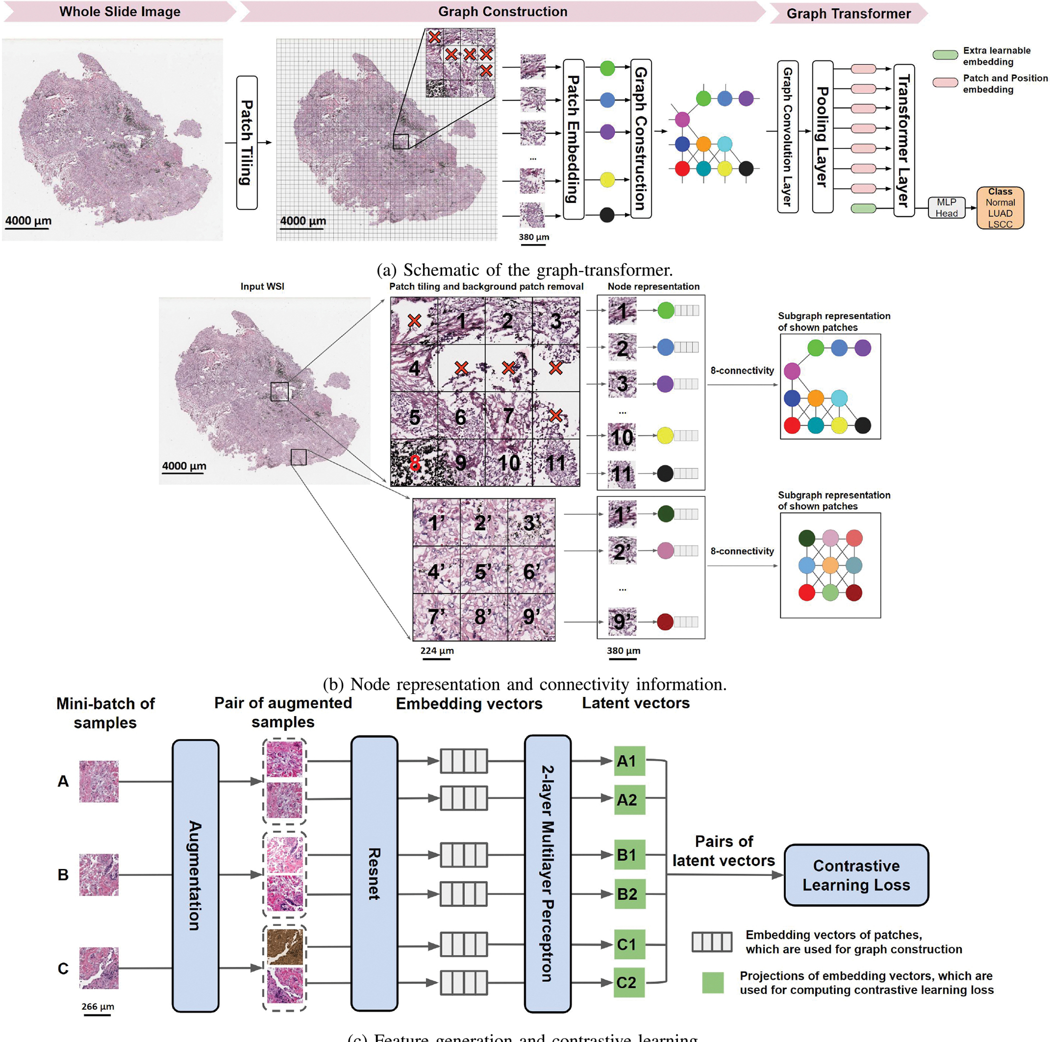
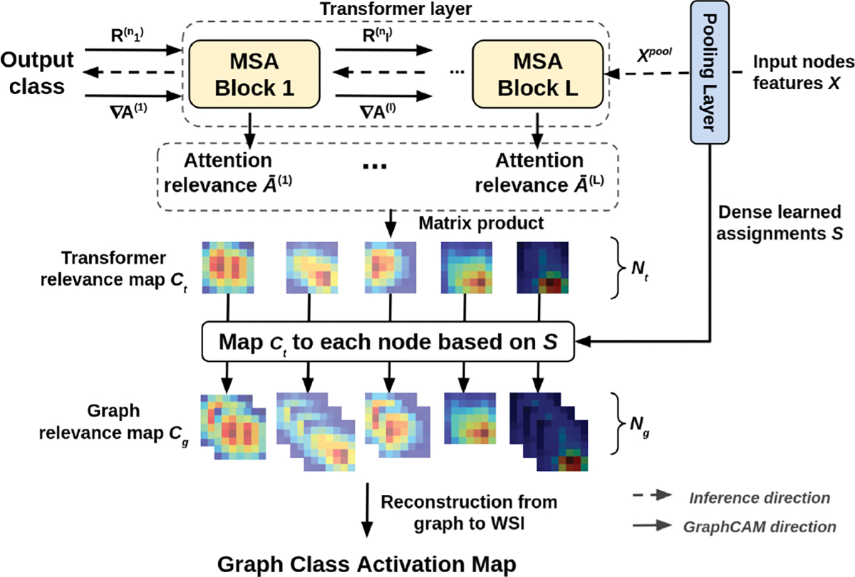
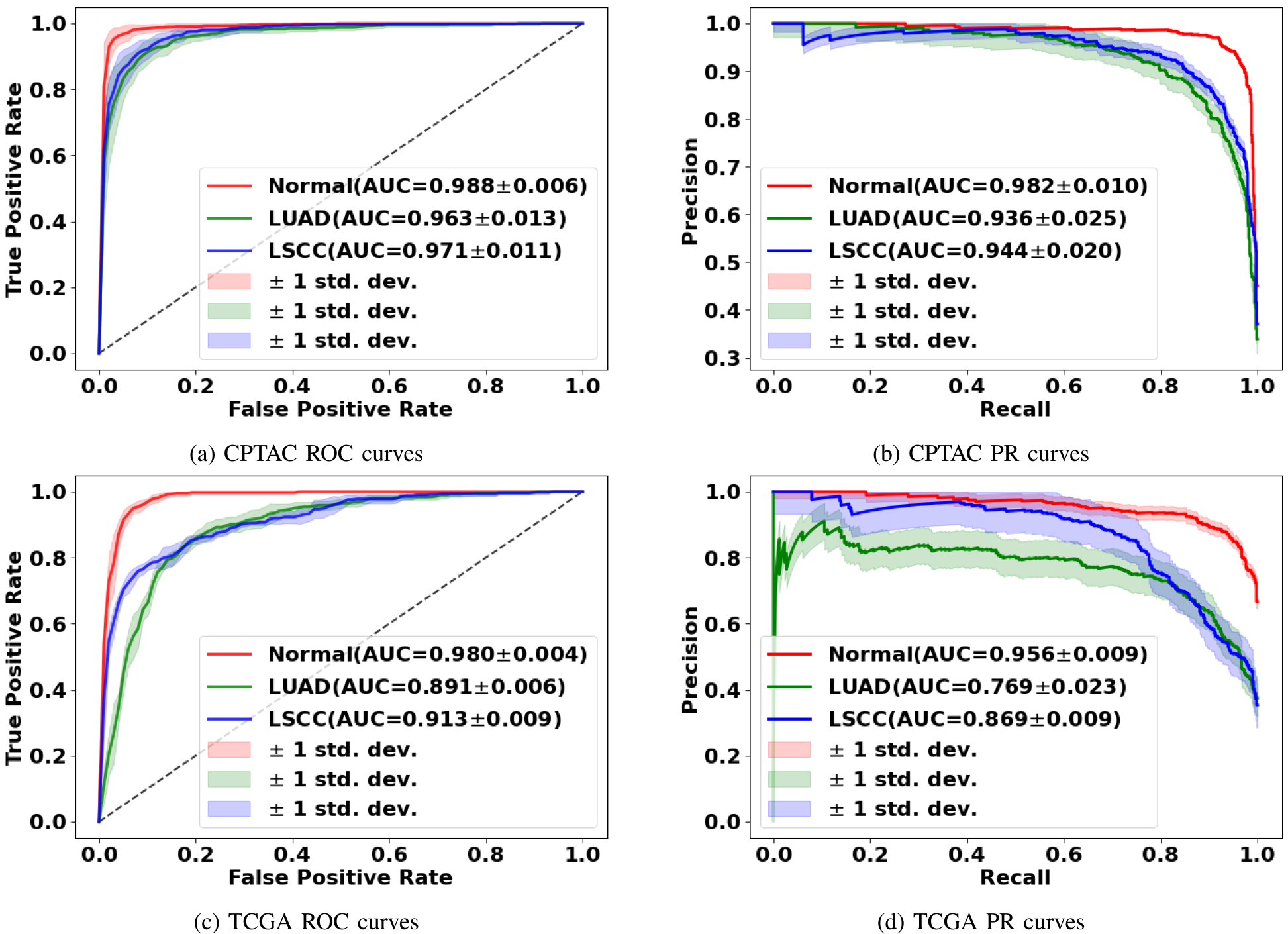
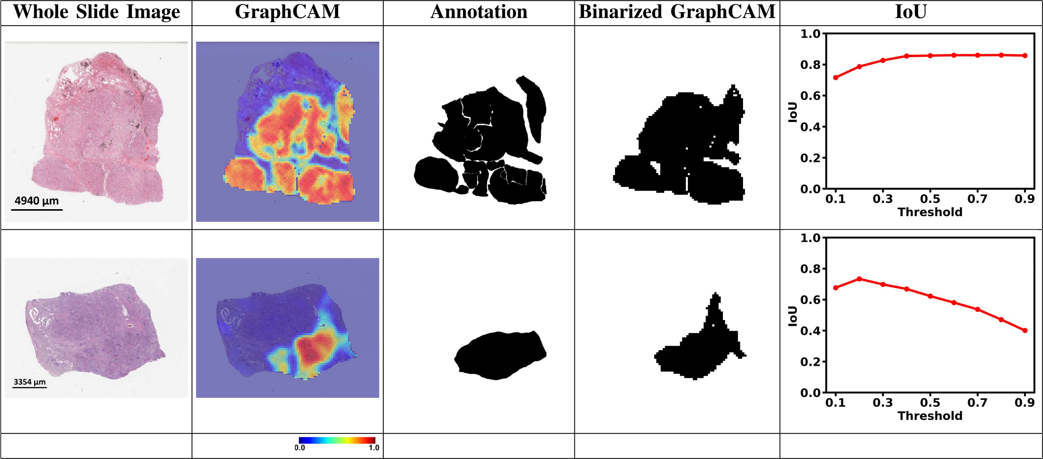
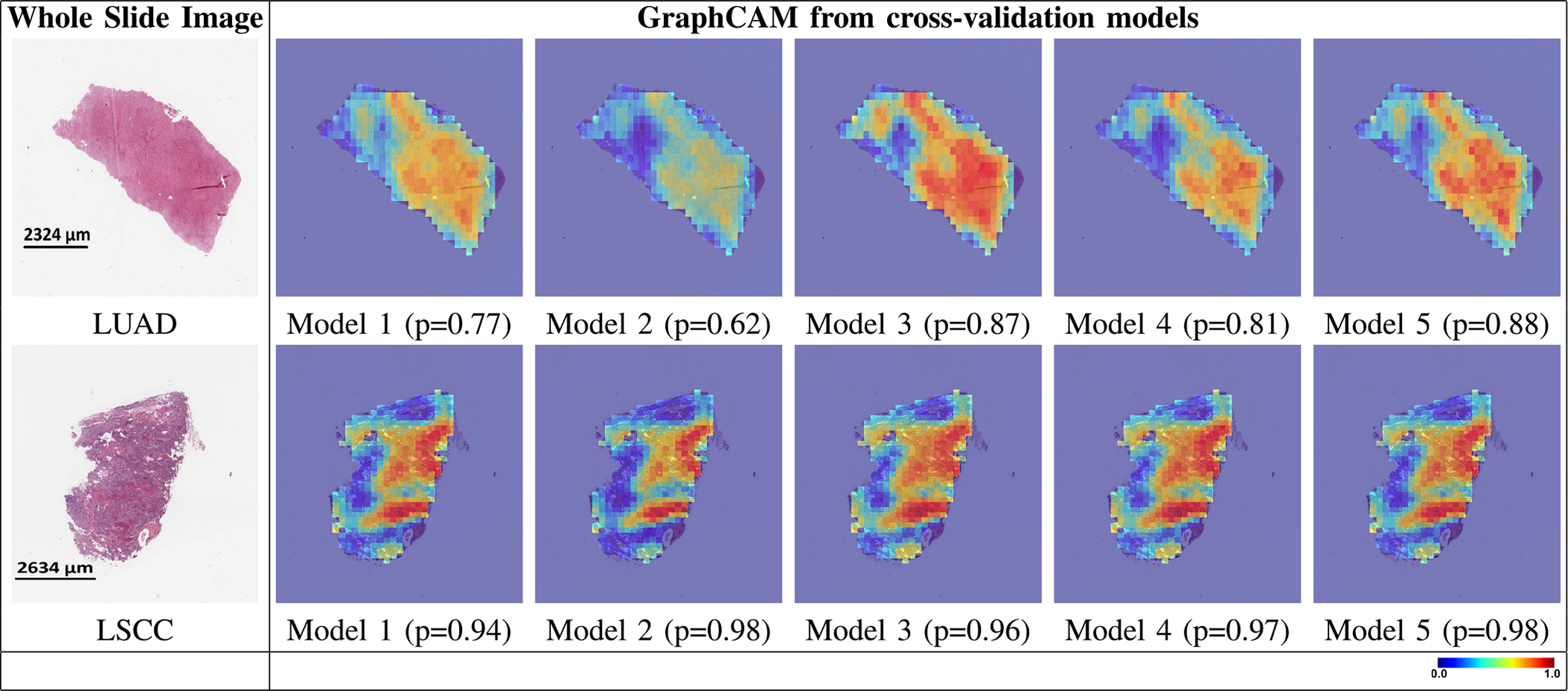
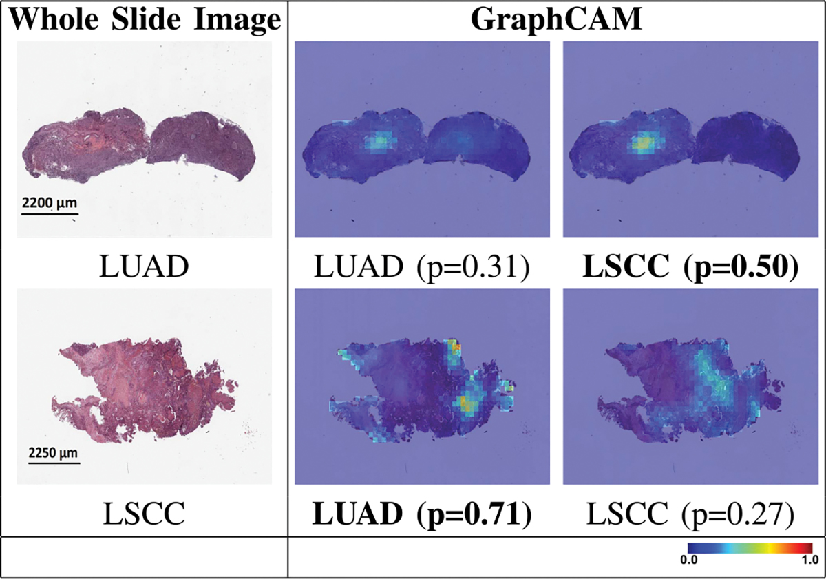
Deep learning is a powerful tool for whole slide image (WSI) analysis. Typically, when performing supervised deep learning, a WSI is divided into small patches, trained and the outcomes are aggregated to estimate disease grade. However, patch-based methods introduce label noise during training by assuming that each patch is independent with the same label as the WSI and neglect overall WSI-level information that is significant in disease grading. Here we present a Graph-Transformer (GT) that fuses a graph-based representation of an WSI and a vision transformer for processing pathology images, called GTP, to predict disease grade. We selected 4,818 WSIs from the Clinical Proteomic Tumor Analysis Consortium (CPTAC), the National Lung Screening Trial (NLST), and The Cancer Genome Atlas (TCGA), and used GTP to distinguish adenocarcinoma (LUAD) and squamous cell carcinoma (LSCC) from adjacent non-cancerous tissue (normal). First, using NLST data, we developed a contrastive learning framework to generate a feature extractor. This allowed us to compute feature vectors of individual WSI patches, which were used to represent the nodes of the graph followed by construction of the GTP framework. Our model trained on the CPTAC data achieved consistently high performance on three-label classification (normal versus LUAD versus LSCC: mean accuracy = 91.2 ± 2.5%) based on five-fold cross-validation, and mean accuracy = 82.3 ± 1.0% on external test data (TCGA). We also introduced a graph-based saliency mapping technique, called GraphCAM, that can identify regions that are highly associated with the class label. Our findings demonstrate GTP as an interpretable and effective deep learning framework for WSI-level classification.

Fig. 1.. The GTP framework.

(a) Each whole slide image (WSI) was divided into patches. Patches that predominantly contained the background were removed, and the remaining patches were embedded in feature vectors by a contrastive learning-based patch embedding module. The feature vectors were then used to build the graph followed by a transformer that takes the graph as the input and predicts WSI-level class label. (b) Each selected patch was represented as a node and a graph was constructed on the entire WSI using the nodes with an 8-node adjacency matrix. Here, two sets of patches of an WSI and their corresponding subgraphs are shown. The subgraphs are connected within the graph representing the entire WSI. (c) We applied three distinct augmentation functions, including random color distortions, random Gaussian blur, and random cropping followed by resizing back to the original size, on the same sample in a mini-batch. If the mini-batch size is K, then we ended up with 2 × K augmented observations in the mini-batch. The ResNet received an augmented image leading to an embedding vector as the output. Subsequently, a projection head was applied to the embedding vector which produced the inputs to contrastive learning. The projection head is a multilayer perceptron (MLP) with 2 dense layers. In this example, we considered K = 3 samples in a minibatch (A, B & C). For sample A, the positive pairs are (A1, A2) and (A2, A1), and the negative pairs are (A1, B1), (A1, B2), (A1, C1), (A1, C2). All pairs were used for computing contrastive learning loss to train the Resnet. After training, we used the embedding vectors (straight from the ResNet) for constructing the graph.

Fig. 2.. Schematic of the GraphCAM.

Gradients and relevance are propagated through the network and integrated with an attention map to produce the transformer relevancy maps. Transformer relevancy maps are then mapped to graph class activation maps via reverse pooling.

Fig. 3.. Model performance on the CPTAC and TCGA datasets.

Mean ROC and PR curves along with standard deviations for the classification tasks (normal vs. tumor; LUAD vs. others; LSCC vs. others) are shown.

Fig. 4.. GraphCAMs and their comparison with the expert annotations.

For each WSI, we generated GraphCAMs and compared them with annotations from the pathologist. The first column contains the original WSIs, the second and third columns contain GraphCAMs and pathologist’s annotations, respectively and the fourth column contains the binarized GraphCAMs based on the threshold from the Intersection of Union (IoU) plot in the last column. The first row shows an LUAD case and the second row denotes an LSCC case.

Fig. 5.. Graph class activation map performance.

GraphCAMs generated on WSIs across the runs performed via 5-fold cross validation are shown. The first column shows the original WSIs and the other columns show the GraphCAMs with prediction probabilities on the cross-validated model runs. The first row shows a sample WSI from the LUAD class and the second row shows an WSI from the LSCC class. The colormap represents the probability by which an WSI region is associated with the output label of interest.

Fig. 6.. GraphCAMs for failure cases.

The first row shows a sample WSI from the LUAD class where the model prediction was LSCC, and the second row shows an WSI from the LSCC class where the model prediction was LUAD. The first column shows the original WSI, and the second and third columns show the generated GraphCAMs along with prediction probabilities. The bold font underneath certain GraphCAMs was used to indicate the model predicted class label for the respective cases. Since this is a 3-label classification task (normal vs. LUAD vs. LSCC), the LUAD and LSCC probability values do not add up to 1.

References

1. Louis DN et al., “Computational pathology: An emerging definition,” Arch. Pathol. Lab. Med, vol. 138, no. 9, pp. 1133–1138, Sep. 2014. - PubMed
1. Louis DN et al., “Computational pathology: A path ahead,” Arch. Pathol. Lab. Med, vol. 140, no. 1, pp. 41–50, 2015. - PMC - PubMed
1. Abels E et al., “Computational pathology definitions, best practices, and recommendations for regulatory guidance: A white paper from the digital pathology association,” J. Pathol, vol. 249, no. 3, pp. 286–294, Nov. 2019. - PMC - PubMed
1. Fuchs TJ and Buhmann JM, “Computational pathology: Challenges and promises for tissue analysis,” Computerized Med. Imag. Graph, vol. 35, nos. 7–8, pp. 515–530, Oct./Dec. 2011. - PubMed
1. Wang X et al., “Weakly supervised deep learning for whole slide lung cancer image analysis,” IEEE Trans. Cybern, vol. 50, no. 9, pp. 3950–3962, Sep. 2020. - PubMed
Publication types