Quantifying nanoscale forces using machine learning in dynamic atomic force microscopy

Abstract

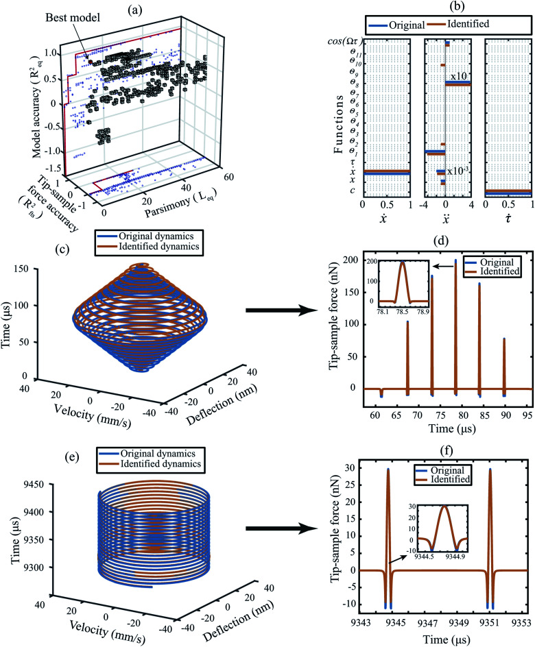
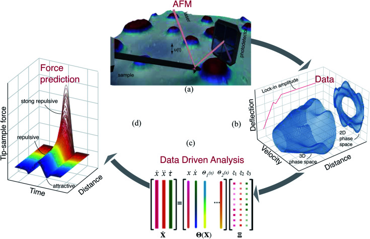
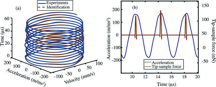
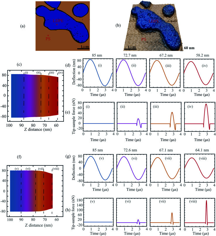
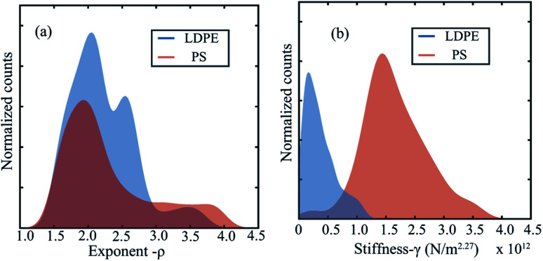
Dynamic atomic force microscopy (AFM) is a key platform that enables topological and nanomechanical characterization of novel materials. This is achieved by linking the nanoscale forces that exist between the AFM tip and the sample to specific mathematical functions through modeling. However, the main challenge in dynamic AFM is to quantify these nanoscale forces without the use of complex models that are routinely used to explain the physics of tip-sample interaction. Here, we make use of machine learning and data science to characterize tip-sample forces purely from experimental data with sub-microsecond resolution. Our machine learning approach is first trained on standard AFM models and then showcased experimentally on a polymer blend of polystyrene (PS) and low density polyethylene (LDPE) sample. Using this algorithm we probe the complex physics of tip-sample contact in polymers, estimate elasticity, and provide insight into energy dissipation during contact. Our study opens a new route in dynamic AFM characterization where machine learning can be combined with experimental methodologies to probe transient processes involved in phase transformation as well as complex chemical and biological phenomena in real-time.

Fig. 1. Training the algorithm on numerically generated data obtained for a cantilever with DMT force model described in ESI Section S1. (a) 3D pareto frontier with parsimony, accuracy of the predicted model, and the tip–sample force as the selection parameters. The blue dots indicate the projection of the 3D cubes onto 2D planes. In the (x, z) plane the red line indicates the pareto optimal line between parsimony and the model accuracy; whereas, in the (x, y) plane it is the optimal line between the parsimony and the tip–sample force accuracy. The best model in this 3D space is highlighted by a red cube. (b) Coefficient matrix showing the influence of each library function on the governing equations. The blue color indicates the original value of the coefficients and the orange color indicates the coefficients as determined by the data-driven algorithm. The description of the functions are given in Table 1. (c and d) Transient dynamics prediction: comparison of the state vectors and the tip–sample force between the DMT simulation (blue) and the data-driven model (orange). (e and f) Steady-state response prediction: comparison of the state vectors and the tip–sample force between the DMT simulation (blue) and the data-driven model (orange). Additional details on selection of hyper-parameters and constraints on the optimization are provided in the Methods section.

Fig. 2. Schematic of the identification process. (a) Experimental data is obtained directly from the photodetector of the AFM. (b) The data is captured using an FPGA device and post-processed to create state vector channels. (c) The state vectors are used as inputs in the sparse identification algorithm to discover the governing model of the system. (d) The data-driven model is used to estimate the tip–sample interaction force.

Fig. 3. Data-driven identification for a silicon cantilever interacting with PS sample. The experimental deflection is obtained at a fixed tip–sample distance of 66 nm (a) identification of velocity and acceleration state vectors. The blue and orange curves represent the experimental and identified state space trajectories, respectively. (b) Estimation of the tip–sample force from data-driven model (orange) superimposed on the experimental acceleration signal (blue).

Fig. 4. Data-driven identification of tip–sample interaction as a function of tip–sample separation on PS-LDPE sample. (a and b) Phase and topography images of PS-LDPE blend sample, respectively. The blue contour indicates the LDPE islands and the orange contour the PS matrix. (c) Experimental dynamic spectroscopy signal obtained with 80% set-point ratio on LDPE material. The dashed lines indicate specific tip–sample distances at which data-driven identification is performed. The distances as read from left to right are at 85 nm, 72.7 nm, 67.2 nm, 58.2 nm, respectively. (d) Experimental deflection signal obtained from averaging 15 periods at different tip–sample sample distances. (e) Identification of tip–sample force based on the data-driven model at different tip–sample distances. (f) Experimental dynamic spectroscopy signal obtained with 80% set-point ratio on PS material. The dashed lines indicate specific tip–sample distances at which data-driven identification is performed. The distances as read from left to right are at 85 nm, 72.6 nm, 67.1 nm, 64.1 nm, respectively. (g) Experimental deflection signal obtained from averaging 15 periods at different tip–sample distances. (h) Identification of the tip–sample force based on data-driven model at different tip–sample sample distances.

Fig. 5. Histograms of conservative tip–sample interaction measurements on PS-LDPE sample. (a) Histograms of the interaction geometry for the PS (red) and LDPE (blue) domains of the sample. (b) Histograms of the stiffness factor for the PS (red) and LDPE (blue) domains of the sample assuming the mean interaction geometry factor of 2.27. The histograms confirm that the PS sample is stiffer than LDPE sample.