Estimating the COVID-19 infection fatality ratio accounting for seroreversion using statistical modelling

Abstract

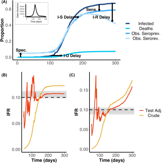
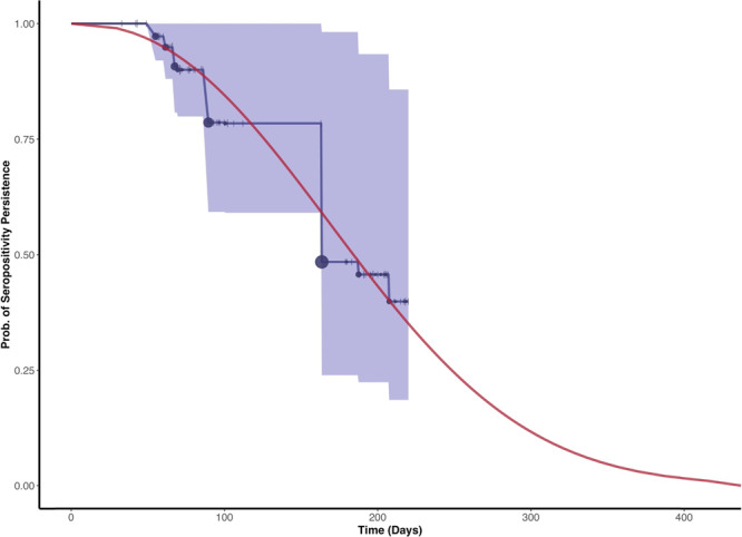
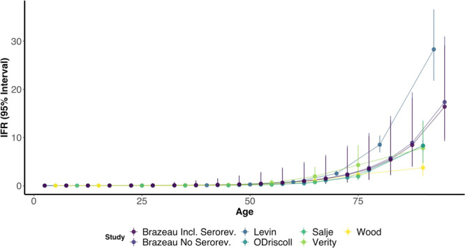
Background: The infection fatality ratio (IFR) is a key statistic for estimating the burden of coronavirus disease 2019 (COVID-19) and has been continuously debated throughout the COVID-19 pandemic. The age-specific IFR can be quantified using antibody surveys to estimate total infections, but requires consideration of delay-distributions from time from infection to seroconversion, time to death, and time to seroreversion (i.e. antibody waning) alongside serologic test sensitivity and specificity. Previous IFR estimates have not fully propagated uncertainty or accounted for these potential biases, particularly seroreversion.

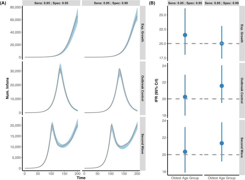
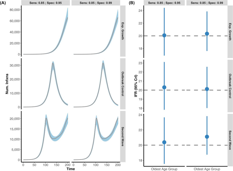
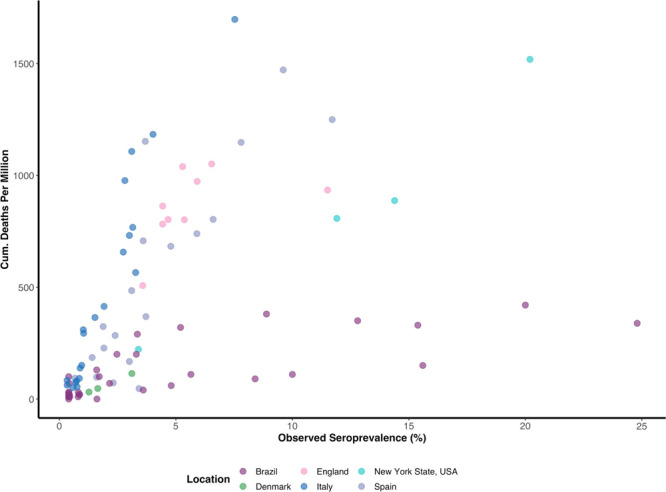
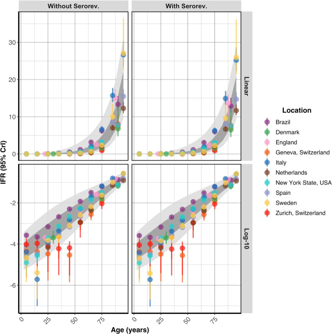
Methods: We built a Bayesian statistical model that incorporates these factors and applied this model to simulated data and 10 serologic studies from different countries.

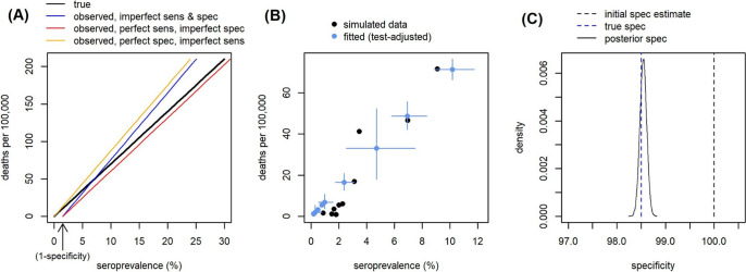
Results: We demonstrate that seroreversion becomes a crucial factor as time accrues but is less important during first-wave, short-term dynamics. We additionally show that disaggregating surveys by regions with higher versus lower disease burden can inform serologic test specificity estimates. The overall IFR in each setting was estimated at 0.49-2.53%.

Conclusion: We developed a robust statistical framework to account for full uncertainties in the parameters determining IFR. We provide code for others to apply these methods to further datasets and future epidemics.

Keywords: Computational biology and bioinformatics; Respiratory tract diseases.

Fig. 1. IFR estimates from serologic data.

A Schematic showing cumulative infections, deaths and seroprevalence with and without seroreversion over time. We highlight the effects of delays from infection to seroconversion (I–S Delay), to death (I–D Delay), and to seroreversion (I–R Delay) as well as serologic test sensitivity (Sens.), serologic test specificity (Spec.) on the observed data. The daily infection curve used as input for the simulation is shown as the plot inset. Early in the outbreak, false positives dominate due to low prevalence and imperfect specificity, whilst later the difference between true cumulative incidence and observed seroprevalence is mainly due to low sensitivity and/or seroreversion. The delays show how the cumulative infection curve is lagged behind the observed seroprevalence. Similarly, the contrast of the seroprevalence curve with (Obs serorev) and without (Obs seroprev) seroreversion reveals the loss of sensitivity over time. These simulations were used as the inputs for the results displayed in (B, C). We used 0.1% of the simulated data at random (i.e. we do not assume we observe the entire population through time). B Estimated IFR over time based on a simulated epidemic that does not include seroreversion. Here, the simulated IFR value is indicated by the dashed black line and the grey lines indicate 100 posterior draws from the fitted statistical model (based on the posterior probability), indicating the capacity for our model framework to correctly recover the true IFR. Red and yellow lines represent the simple and test-adjusted (Rogan-Gladen correction) IFR estimates (see Main Text), calculated as if the serosurvey had been conducted on each respective day (after day 50). In the case without seroreversion, the IFR appears to be adequately captured by the Rogan-Gladen correction once infections have stopped accruing (the realised IFR appears to be slightly greater than the initial simulated true IFR value of 0.1). C As for (B), but the simulation and statistical model both include seroreversion. The IFR values are shown as a probability. In the case that includes seroreversion, the Rogan-Gladen correction can no longer adequately capture the IFR value, as seroprevalence estimates are constantly changing. In addition, in the outbreak, when the true seroprevalence is less than the false positive rate, adjusting for the serologic test characteristics can result in unstable IFR estimates.

Fig. 2. Posterior daily infections and IFR estimates from simulated data without seroreversion.

A Using simulated data, we created three outbreak scenarios where individuals who seroconverted could not serorevert: exponential growth, outbreak control, and second wave (grey lines are simulated infection input) under two different serologic tests (Sensitivity: 85%; Specificity 95% vs. Sensitivity: 85%; Specificity 99%). The blue shading represents 100 posterior draws of the modelled infection curve, where draws were selected based on their posterior probability. B The inferred median and 95% credible intervals (blue) versus the simulated true IFR (grey, dashed line) with two different serologic tests, in the oldest age group. For all epidemic scenarios considered, we assume that there are two seroprevalence surveys that range over days 120–130 and 170–180 and that 0.1% of the population was sampled.

Fig. 3. Posterior daily infections and IFR estimates from simulated data with seroreversion.

A Three simulated epidemics were generated (exponential growth, outbreak control, and second wave) as in Fig. 2, but now with the additional feature that individuals who seroconverted would eventually serorevert. Grey lines indicate the simulated true infection curve under two different serologic tests (Sensitivity: 85%; Specificity 95% vs. Sensitivity: 85%; Specificity 99%). The blue shading represents 100 posterior draws (based on the posterior probability) of the modelled infection curve (using an exponentiated natural cubic spline), where draws were selected based on their posterior probability. B The inferred median and 95% credible intervals (blue) versus the simulated true IFR (grey, dashed line) in the oldest age group for each of the outbreak scenarios with respect to the two different serologic test characteristics. As above, the model accurately captures both the simulated infection curve and the simulated IFR while accounting for seroreversion. For all epidemic scenarios considered, we assume that there are two seroprevalence surveys that range over days 120–130 and 170–180 and that 0.1% of the population was sampled.

Fig. 4. Estimating serologic test specificity from regional data.

A Expected relationship between seroprevalence and deaths per 100,000 under different values of serologic test sensitivity and specificity, when overall IFR = 0.7% and both IFR and population age structure are constant. B Example simulation of seroprevalence and deaths per 100,000 in different regions within a serosurvey (black), assuming varying burden of COVID-19 and population sizes between regions, but constant test performance and IFR. Model-estimated mortality and seroprevalence (adjusted for test performance) for each region when fitting to the simulated data (blue; error bars = 95% CrI). Serologic test performance is simultaneously estimated by the model, using informative priors from a simulated validation study and the relationship between seroprevalence and mortality. C Initial prior specificity estimate based on a simulated validation study including 100 true negative cases (black dashed line); by chance 100% specificity was measured in the simulated validation study, although the true value is 98.5% (blue dashed line). The model fitted to simulated regional data is able to infer a much more accurate posterior specificity estimate (black solid line shows posterior distribution).

Fig. 5. Seroreversion data and model fit.

Persistence of seropositive test results with the Abbott assay among an extended cohort of 101 COVID-19 patients (extended dataset based from Muecksch et al.). The interval-censored Kaplan–Meier survival curve with 95% confidence intervals (blue) with censored observations (ticks) and seroreversion events (circles) is shown for comparison. Both censoring (range 1–4) and seroreversion events (range 0–16.16) are scaled according to the number of observations on the given day. The fitted Weibull survival function (red) of persistence of a serologic positive result is shown in red. The fit was estimated from symptom onset to time of seroreversion, where the time of seroreversion was estimated incorporating interval censoring. The mean time from symptom onset to seroreversion was 190.93 days.

Fig. 6. First-wave data: mortality versus seroprevalence.

Relationship between seroprevalence and COVID-19 mortality per 1,000,000 among surveys which could be broken down by region.

Fig. 7. Age-stratified infection fatality ratio estimate.

The age-specific modelled IFR (%) median and 95% credible interval estimates with and without seroreversion are plotted on a linear and log-10 scale (mean age within each age group plotted). The 95% prediction intervals (light grey) and the 80% prediction intervals (dark grey) calculated from the age-specific pooled-IFR estimates are shown for each model. The IFR increases in a log-linear fashion with age.

Fig. 8. Comparison of age-specific COVID-19 IFR estimates during the first-wave.

We compare estimates from the current study (Brazeau; including seroversion (Incl. Serorev.) vs. excluding seroreversion (No Serorev.)) with and without seroreversion, Levin et al., Salje et al., Wood et al., O’Driscoll et al. and Verity et al.. Of note, studies used different statistical (i.e. frequentist versus bayesian) and methodological approaches that make the 95% confidence or credible intervals not directly comparable.

References

1. Meyerowitz-Katz G, Merone L. A systematic review and meta-analysis of published research data on COVID-19 infection fatality rates. Int. J. Infect. Dis. 2020;101:138–148. doi: 10.1016/j.ijid.2020.09.1464. - DOI - PMC - PubMed
1. O’Driscoll M, et al. Age-specific mortality and immunity patterns of SARS-CoV-2. Nature. 2021;590:140–145. doi: 10.1038/s41586-020-2918-0. - DOI - PubMed
1. Ioannidis JPA. Infection fatality rate of COVID-19 inferred from seroprevalence data. Bull. World Health Organ. 2021;99:19–33F. doi: 10.2471/BLT.20.265892. - DOI - PMC - PubMed
1. Verity, R. et al. Estimates of the severity of coronavirus disease 2019: a model-based analysis. Lancet Infect. Dis. 10.1016/S1473-3099(20)30243-7 (2020). - PMC - PubMed
1. Wood, S. N., Wit, E. C., Fasiolo, M. & Green, P. J. COVID-19 and the difficulty of inferring epidemiological parameters from clinical data. Lancet Infect. Dis. 10.1016/S1473-3099(20)30437-0 (2020). - PMC - PubMed