Comprehensive assessment of differential ChIP-seq tools guides optimal algorithm selection

Abstract

Background: The analysis of chromatin binding patterns of proteins in different biological states is a main application of chromatin immunoprecipitation followed by sequencing (ChIP-seq). A large number of algorithms and computational tools for quantitative comparison of ChIP-seq datasets exist, but their performance is strongly dependent on the parameters of the biological system under investigation. Thus, a systematic assessment of available computational tools for differential ChIP-seq analysis is required to guide the optimal selection of analysis tools based on the present biological scenario.

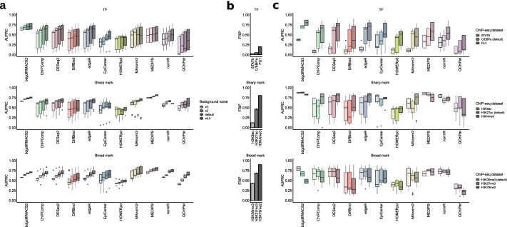
Results: We created standardized reference datasets by in silico simulation and sub-sampling of genuine ChIP-seq data to represent different biological scenarios and binding profiles. Using these data, we evaluated the performance of 33 computational tools and approaches for differential ChIP-seq analysis. Tool performance was strongly dependent on peak size and shape as well as on the scenario of biological regulation.

Conclusions: Our analysis provides unbiased guidelines for the optimized choice of software tools in differential ChIP-seq analysis.

Keywords: Benchmarking differential ChIP-seq tools; Bioinformatic analysis; Differential ChIP-seq; Guidelines for differential ChIP-seq.

Fig. 1

Simulation and sub-sampling of differential ChIP-seq experiments. a Schematic overview of simulated peaks and regulation scenarios: Each box represents one test scenario, per scenario the compared samples, and their signal strength are shown in blue and in red. The columns show transcription factor (TF), H3K27ac (sharp mark) and H3K36me3 (broad mark) histone mark ChIP-seq signals (DCSsim width parameters shown below). In the 50:50 regulation scenario, the number of differential regions is equally distributed, while in the 100:0 scenario we assume a global downregulation of the signal. Arrow positions indicate the differential ChIP-seq signals and their color show the sample with the higher signal. b Overview of the benchmarking workflow. We applied DCSsim to simulate in silico data and DCSsub to sub-sample genuine ChIP-seq signals. This resulted in sequence reads for two samples (red and blue). After preprocessing, we directly applied peak-independent tools or peak-dependent DCS tools subsequent to peak calling. The resulting peaks and differential regions are depicted as arrows. To assess the DCS tools, we calculated the area under the precision-recall curves. c Heatmaps and profile plots showing all peak regions of a ChIP-seq experiment for the TF C/EBPa (left), DCSsub sub-sampling from the same dataset (middle), and the DCSsim simulation of TF peak shapes (right). d Quantitative overview of test cases. We generated five independent datasets per peak-regulation scenario. Then we applied three peak callers in combination with 12 peak-dependent DCS tools and 21 peak-independent DCS tools. We used up to 16 parameter setups per DCS tool, and analyses were run for simulated and sub-sampled ChIP-seq data. * HOMER with previously called peaks (HOMERpd)

Fig. 2

Performance of simulated and sub-sampled input data. a Log2-fold change of AUPRC values obtained from DCSsim simulated and DCSsub sub-sampled data. Values >0 indicate a better performance based on AUPRC for simulated data and <0 indicates a higher AUPRC for sub-sampled input. The overall difference for all DCS tools is shown on the left (bar with gray background). Tools were ordered by their median log2-fold change. b Comparison of AUPRC values of simulated and sub-sampled data for peak-dependent (n = 431) vs. peak-independent (n = 1363) DCS tools. P-value two-sided Wilcoxon rank sum test. Box plot limits, 25% and 75% quantiles; center line, median; whiskers, 1.5× interquartile range

Fig. 3

Performance of benchmarked DCS tools based on AUPRC values. a Overview of AUPRC values per DCS tool for all test scenarios compared to random regions (see “Methods”), ranked by median AUPRC. Box plot limits, 25% and 75% quantiles; center line, median; whiskers, 1.5× interquartile range. b Density plots of AUPRC values per scenario for TFs (left), sharp (middle), and broad marks (right). The two (one for each regulation scenario) top-performing parameter sets per DCS tool are highlighted as colored symbols, remaining data points are visualized as density clouds. c AUPRC values of the top five DCS tools parameter sets per scenario (TF left, sharp mark middle, and broad mark right column; 50:50 regulation scenario top and 100:0 bottom row). Colored boxes indicate peak caller, if applicable and if default or adjusted parameter setups were used; whiskers, standard error of the mean

Fig. 4

Accuracy profiles of DCS tools. a Schematic representation of accuracy profiles. Rows with yellow background show simulated or sub-sampled ChIP-seq signals. The reference region highlights the sample color with the higher signal. Regions with no difference are depicted in gray. The predicted regions from a DCS tool are highlighted with green and the calculated accuracy metrics with blue background. We investigated false positives, false negatives, and too long and too short regions, representing the false positive and false negative base pairs (bp), respectively with the constraint that the predicted regions overlapped with a reference region. b Bar charts show the false discovery rate (FDR), the false omission rate (FOR), the percentage of too short, and the percentage of too long bp for the best-performing parameter sets of the top 5 DCS tool parameter combinations per scenario (from left/5th to the right/1st) based on AUPRC. TFs (left), sharp marks (middle), and broad marks (right) in the columns and 50:50 regulation (top) as well as 100:0 regulation (bottom) in the rows. Whiskers represent the standard deviation. c Example coverage plot of DCSsub sub-sampled H3K27ac reads (samples in row 1 (red) and 2 (blue)) representing sharp marks with the respective reference regions (row 3). In row 3 upregulation in sample 1 is indicated in red, downregulation in blue. Rows 4 to 8 show predicted regions from the best parameter setups of the top 5 DCS tools for sharp mark data and 50:50 regulation. The height of predicted regions represents the − log10 of p-value, adjusted p-value, or FDR or the score derived from the respective DCS tool. Higher bars represent higher confidence in the indicated region

Fig. 5

Influence of FRiP on the performance of DCS tools. a AUPRCs of the top 11 DCS tools (based on AUPRC for the initial six shape and regulation scenarios) depend on the background noise. Boxplots per DCS tool are ordered by noise level, from high to low. b FRiP in the sub-sampled datasets. Darker color represents higher FRiP. Top panel, TFs; middle panel, sharp marks; bottom panel, broad marks. Whiskers indicate the standard deviation. c AUPRCs for sub-sampled ChIP-seq data from different TFs and histone marks depend on FRiP. Boxplots per DCS tool are ordered by FRiP from low to high. Top panels, TFs; middle panels, sharp marks; bottom panels, broad marks. Box plot limits, 25% and 75% quantiles; center line, median; whiskers, 1.5× interquartile range

Fig. 6

Chromosome characteristics and signal distribution influence AUPRC. Combined AUPRCs from simulated and sub-sampled data of the top 11 DCS tools (based on AUPRC of the initial six shape and regulation scenarios) for five chromosomes of mm10 (chr1, chr8, chr11, chr19, and chrX) for TFs, sharp, and broad marks are shown. Chromosomes per DCS tool are ordered by length, from short to long. Top panel, TFs; middle panel, sharp marks; bottom panel, broad marks. Box plot limits, 25% and 75% quantiles; center line, median; whiskers, 1.5× interquartile range

Fig. 7

Runtime and memory requirements of benchmarked DCS tools. a Average runtime and b memory consumption of all benchmarked DCS tools over the six tested scenarios. Due to their extensive runtimes, GenoGAM and MultiGPS were executed with 5 workers. Whiskers indicate standard error of the mean

Fig. 8

DCS tool performance and guidelines for DCS tool selection. a Heatmap summarizing DCS tool performance. Columns represent top AUPRC values, accuracy profiles, stability, runtime, memory consumption, and mean DCS score of the benchmarked DCS tools. The AUPRC of the best parameter setup per DCS tool is shown for peak shape and regulation scenarios and their respective combinations. All other metrics are shown as average of all parameter setups per DCS tool over all test scenarios. Standard deviations were calculated between AUPRCs of the simulated and sub-sampled replicates. The number of NA results summarizes all failed and faulty execution runs or runs with empty outputs. Preparation time represents the time to process the input files preceding DCS prediction. Tools were ordered by their mean DCS score over all test sets. b, c Decision trees listing top-performing parameter setups per DCS tool based on DCS score to guide investigators towards the five top-ranking DCS tools and their parameter setups depending on peak shape and regulation scenario. c Decision tree for situations where shape, regulation, or both are unknown. Here, the ranking is based on DCS score of the combined regulation scenarios for TFs, sharp, and broad marks, the combined peak shapes for 50:50 and 100:0 regulation and over all tested scenarios for situations where shape and regulation are unknown. Colored boxes indicate the applied peak caller for the respective parameter setup and if default, default with custom windows, or adjusted parameters should be used. For detailed information on the setups, see Additional file 4: Table S3 and Additional file 6: Table S5

References

1. Johnson DS, Mortazavi A, Myers RM, Wold B. Genome-wide mapping of in vivo protein-DNA interactions. Science. 2007;316(5830):1497–1502. doi: 10.1126/science.1141319. - DOI - PubMed
1. Robertson G, Hirst M, Bainbridge M, Bilenky M, Zhao Y, Zeng T, et al. Genome-wide profiles of STAT1 DNA association using chromatin immunoprecipitation and massively parallel sequencing. Nat Methods. 2007;4(8):651–657. doi: 10.1038/nmeth1068. - DOI - PubMed
1. Xie W, Schultz MD, Lister R, Hou Z, Rajagopal N, Ray P, et al. Epigenomic analysis of multilineage differentiation of human embryonic stem cells. Cell. 2013;153(5):1134–1148. doi: 10.1016/j.cell.2013.04.022. - DOI - PMC - PubMed
1. Zhu J, Adli M, Zou JY, Verstappen G, Coyne M, Zhang X, et al. Genome-wide chromatin state transitions associated with developmental and environmental cues. Cell. 2013;152(3):642–654. doi: 10.1016/j.cell.2012.12.033. - DOI - PMC - PubMed
1. Ernst J, Kheradpour P, Mikkelsen TS, Shoresh N, Ward LD, Epstein CB, et al. Mapping and analysis of chromatin state dynamics in nine human cell types. Nature. 2011;473(7345):43–49. doi: 10.1038/nature09906. - DOI - PMC - PubMed
Publication types
MeSH terms
LinkOut - more resources