Measuring Cytoskeletal Mechanical Fluctuations and Rheology with Active Micropost Arrays

Abstract

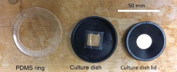
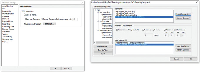
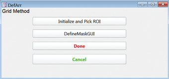
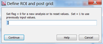
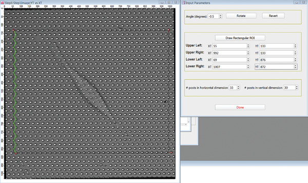
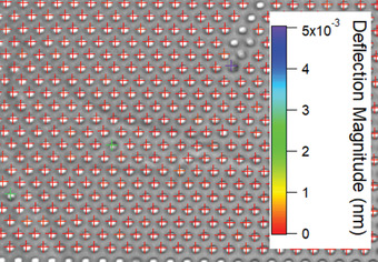
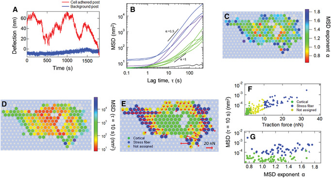
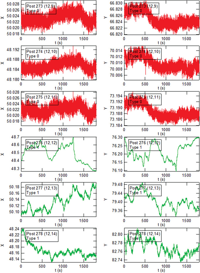
The dynamics of the cellular actomyosin cytoskeleton are crucial to many aspects of cellular function. Here, we describe techniques that employ active micropost array detectors (AMPADs) to measure cytoskeletal rheology and mechanical force fluctuations. The AMPADS are arrays of flexible poly(dimethylsiloxane) (PDMS) microposts with magnetic nanowires embedded in a subset of microposts to enable actuation of those posts via an externally applied magnetic field. Techniques are described to track the magnetic microposts' motion with nanometer precision at up to 100 video frames per second to measure the local cellular rheology at well-defined positions. Application of these high-precision tracking techniques to the full array of microposts in contact with a cell also enables mapping of the cytoskeletal mechanical fluctuation dynamics with high spatial and temporal resolution. This article describes (1) the fabrication of magnetic micropost arrays, (2) measurement protocols for both local rheology and cytoskeletal force fluctuation mapping, and (3) special-purpose software routines to reduce and analyze these data. © 2022 The Authors. Current Protocols published by Wiley Periodicals LLC. Basic Protocol 1: Fabrication of magnetic micropost arrays Basic Protocol 2: Data acquisition for cellular force fluctuations on non-magnetic micropost arrays Basic Protocol 3: Data acquisition for local cellular rheology measurements with magnetic microposts Basic Protocol 4: Data reduction: determining microposts' motion Basic Protocol 5: Data analysis: determining local rheology from magnetic microposts Basic Protocol 6: Data analysis for force fluctuation measurements Support Protocol 1: Fabrication of magnetic Ni nanowires by electrodeposition Support Protocol 2: Configuring Streampix for magnetic rheology measurements.

Keywords: cytoskeleton; magnetic actuation; microposts; microrheology.

Figure 1

Overview of protocols and workflow for local cellular rheology and force fluctuation measurements using AMPADs.

Figure 2

Condenser of Nikon TE‐2000 microscope, showing location of UV and IR filters in the incident light path (glass disks circled in red.).

Figure 3

40× image of a NIH 3T3 cell on a micropost array.

Figure 4

Sample histogram of image intensity after setting halogen illuminator lamp intensity in Streampix prior to data acquisition.

Figure 5

Dual magnetic tweezer system mounted on Nikon T/E 2000 microscope. (A) Microscope in enclosure incubator. (B) Closeup showing tweezer assembly mounted on metal plate (a) over microscope stage. Each of the two magnet assemblies is mounted in an aluminum heat‐sinking block (b) on a 3‐axis micromanipulator (c). (C) Further closeup showing the ends of the magnet solenoids (d) and the tapered iron cores of tweezers (e) projecting over the custom‐built sample dish (f). The dish rests on a heating plate (g) and can be moved with the microscope's sample stage relative to the tweezer tips. (D) Schematic of the sample dish, showing the AMPAD sample location, the tweezer tips (gray), the acetal base (blue) and lid (green) of the dish, and the PDMS ring (yellow) that seals the space for culture media (pink). See text and Figure 7 for further details. Panel C is reproduced from (Shi, 2020). Used by permission. Panel D is reproduced from (Shi et al., 2019).

Figure 6

Block diagram of the measurement system for AC cellular rheology measurements with magnetic microposts. Green arrows: flow of control from PC to camera and magnetic tweezers. Red arrows: flow of image data from camera and magnetic field data from Hall sensors to the PC. Yellow arrow: trigger output from camera to NI card to synchronize the Hall sensor measurements with the image frame capture. Note that the Kepco power supply is operated in current programming mode.

Figure 7

Components of the custom sample dish for cell rheology measurements. The PDMS ring has an outer radius of 55 mm and am inner radius of 45 mm. Reproduced from Ref. (Shi, 2020). Used by permission.

Figure 8

Screenshot of module list in Streampix. Choose VoltageoutNin_sync_DF for active microrheology data acquisition.

Figure 9

Screen shot for setting up the command “Start” under the event “On PostCreate AVI.”

Figure 10

Screen shot for setting up the command “Stop” under the event “On Recording Stopped.”

Figure 11

Screen shot for setting up the command “Increment” under the event “On AVI Image Saved.”

Figure 12

Screen shot for setting up the auto‐naming and file naming convention in the Streampix settings.

Figure 13

Screen shot for use of recording script when imaging.

Figure 14

Main Igor Pro graphical user interface (GUI) for data reduction and analysis.

Figure 15

GUI accessed from “Define Array and Mask” in main GUI. It is used to define the set of posts to be analyzed and provide an initial mask classifying the posts.

Figure 16

Input window in Initialize and Pick ROI to reset ROI or use previous settings.

Figure 17

(A) GUI for setting the ROI centered on the cell to be analyzed and containing the posts to be tracked. After rotating the image so the rows of posts are horizontal, the drawing tools (upper left) are used to define a rectangular ROI. (B) After clicking “Done Drawing,” the positions of the four corners are updated in the GUI and are marked by the red crosses in the image.

Figure 18

Illustration of adjustment of the two crosses at the bottom of the ROI to move them on top of the microposts. The green line indicates the path along which to count the posts in the vertical direction.

Figure 19

GUI for SetMaskPanel to create the initial identification of cell‐associated and background posts, and defective or other posts to be ignored in the analysis. All posts are initially labeled as background posts (red crosses).

Figure 20

Drawing panel to manually draw the cell outline with the IgorPro polygon tool.

Figure 21

View of mask array showing background posts (red crosses), cell posts (Green x) and ignored posts (purple hourglass symbols).

Figure 22

Pop‐up window for “Fit All Posts” button.

Figure 23

Pop‐up window for “Plot A Lot” button to display displacement traces versus time.

Figure 24

Pop‐up window for “Cont fitAllPosts” to determine post displacements versus time for magnetic rheology measurements.

Figure 25

Panels for calculating oscillation amplitudes via digital lock‐in (DLI) from the posts’ deflections. (A) Pop up window when for button “cont double freq” to calculate DLI on all movies taken with different driving frequencies. (B) Pop up window for button “Double freq” to calculate DLI on a specific movie.

Figure 26

Heatmap of digital lock‐in magnitude at f = 0.1 Hz. The color scale shows the deflection magnitude in nm.

Figure 27

Pop‐up window for mean squared displacement (MSD) calculation.

Figure 28

Pop‐up window for “Make Cell Mask MSD” button.

Figure 29

Pop‐up window for “Force Bifurcation” button.

Figure 30

Sample micropost deflection fluctuations for a cardiac myofibroblast (Shi et al., 2021). (A) Deflection trace of one Cartesian component of the motion of a cell‐associated micropost (red) and a background micropost (blue) over 30 min (Basic Protocol 4). (B) MSDs versus lag time τ determined from traces such as those in (A) for the posts indicated by red circles in C. The traces’ color shows the MSD power law exponent α over the range 5 s ≤ τ ≤ 10 s as given by the scale in panel C. The black trace is for the background post shown in A. (C and D) Heat maps of (C) distribution the exponent α over 5 s ≤ τ ≤ 10 s, and (D) the MSD magnitude at τ = 10 s Each hexagon represents a post. Gray hexagons indicate posts that were not coupled with the cell over the full measurement interval. Gray circles show background posts. (E) Distribution of cortical and stress fiber posts across the cell, as determined by the classification procedure based on average traction force magnitude described in Basic Protocol 6, and the corresponding traction force vectors (red arrows). (F) Scatter plot of MSD magnitude at τ = 10 s versus average traction force. (G) MSD magnitude at τ = 10 s versus MSD exponent α for cortical and stress fiber posts.

Figure 31

Measurements of local cellular rheology with magnetic microposts. (A) Deflection of a cortex‐adhered magnetic post, driven by a magnetic field with sinusoidal oscillations at a measurement frequency f = 1 Hz and a reference frequency f_R = 7 Hz. (B) The amplitudes of the responses at the two frequencies vary with time in a correlated way. (C) These temporal variations yield significant noise in the raw measurement of the post displacement amplitude x(ω) (blue symbols). By calculating the ratio x(ω)/x(ω _R) (green symbols), this noise is greatly reduced, thus improving the determination of the frequency dependence of x(ω). (D) Frequency‐dependent apparent stiffness of a post with a cell attached and the same post after removal of the cell. (E) Frequency‐dependent cellular stiffness determined from the data in D.

Figure 32

(A) Raw image frame of micropost array. (B) Corresponding intermediate image following filtering as described in the Commentary.

Figure 33

Subtracted MSD and its logarithmic time derivative, illustrating the determination of the MSD exponent α for two microposts. (A) Raw MSD traces showing fits (red lines) to determine the noise floor as described in the Commentary. (B) MSD traces MSD_Sub after subtracting the noise floor from the raw MSDs. (C) Logarithmic time derivatives of MSD_Sub . The MSD exponent α and its uncertainty were obtained from the average of the logarithmic time derivative in the range 5 s ≤ τ ≤ 10 s. The MSDs were computed at 0.1 s intervals in τ, but above τ = 10 s, they are only plotted every 1 s.

Figure 34

Effects of cell motility on micropost dynamics and identification of microposts that were engaged with a cell over the full 1800 s measurement interval as those whose MSD exponents α₁ and α₃ computed over the first and final thirds of the trajectory, respectively, both be >0.5 (A) A “background” micropost that was not in contact with the cell. (B) A micropost engaged with the cell only in the latter part of the measurement interval. (C) A micropost initially engaged with the cell, but subsequently released. (D) A micropost coupled to the cellular cortex throughout the measurement. (E‐H) MSDs for the first and final thirds of the measurement intervals for the traces shown in A‐D.

Figure 35

Sample field of view for magnetic microposts array. The green circle indicates the location of a magnetic micropost. The two red circles indicate collapsed posts that can be used as navigation aids to trace back to the same location after cell removal.

Figure 36

Raw post trajectory data. X (left column) and Y (right column) coordinates (in camera pixels) of selected posts as determined from particle tracking analysis versus time (in seconds). In these data, 1 pixel = 125 nm. This video was taken at 10 fps, and so includes 18,000 time points. These plots are generated by the “Plot‐a‐lot” function in the associated IgorPro analysis code. The post number is that in the Igor data arrays, and the (a,b) notation references a representation of the hexagonal post lattice in a 2D array. Post type 0 (red) denotes background posts, and Post type 1 (green) denotes cell‐associated posts.

Figure 37

Dedrifted post trajectory data. X (left column) and Y (right column) coordinates (in camera pixels) of the posts shown in Figure 33 following dedrifting versus time (in seconds). In these data, 1 pixel = 125 nm. This video was taken at 10 fps, and so includes 18,000 time points. The plots are generated with the “Plot‐a‐lot” function in the associated IgorPro analysis code. The post number is that in the Igor data arrays, and the (a,b) notation references a representation of the hexagonal post lattice in a 2D array. Post type 0 (red) denotes background posts, and Post type 1 (green) denotes cell‐associated posts.

Figure 38

Micropost deflection data. X (left column) and Y (right column) coordinates (in camera pixels) versus time (seconds) of the posts shown in Figures 33 and 34 following subtraction of the individual posts’ undeflected positions. In these data, 1 pixel = 125 nm. This video was taken at 10 fps, and so includes 18,000 time points. The plots are generated with the “Plot‐a‐lot” function in the associated IgorPro analysis code. The post number is that in the Igor data arrays, and the (a,b) notation references a representation of the hexagonal post lattice in a 2D array. Post type 0 (red) denotes background posts, and Post type 1 (green) denotes cell‐associated posts.

Figure 39

X‐component of deflection data in nm versus time for cell post 278 and background post 273 from Figure 33. The right‐hand vertical axis shows the conversion to traction force, based on the posts’ spring constant k = 15.7 nN/µm.

References

1. Alencar, A. M. , Ferraz, M. S. A. , Park, C. Y. , Millet, E. , Trepat, X. , Fredberg, J. J. , & Butler, J. P. (2016). Non‐equilibrium cytoquake dynamics in cytoskeletal remodeling and stabilization. Soft Matter, 12(41), 8506–8511. doi: 10.1039/c6sm01041e - DOI - PMC - PubMed
1. Bose, P. , Huang, C. Y. , Eyckmans, J. , Chen, C. S. , & Reich, D. H. (2018). Fabrication and mechanical properties measurements of 3D microtissues for the study of cell‐matrix interactions Methods in Molecular Biology, 1722, 303–328. doi: 10.1007/978-1-4939-7553-2_18 - DOI - PubMed
1. Crocker, J. C. , & Grier, D. G. (1996). Methods of digital video microscopy for colloidal studies. Journal of Colloid and Interface Science, 179(1), 298–310. doi: 10.1006/jcis.1996.0217 - DOI
1. Dixon, P. K. , & Wu, L. (1989). Broad‐band digital lock‐in amplifier techniques. Review of Scientific Instruments, 60(10), 3329–3336. doi: 10.1063/1.1140523 - DOI
1. du Roure, O. , Saez, A. , Buguin, A. , Austin, R. H. , Chavrier, P. , Siberzan, P. , & Ladoux, B. (2005). Force mapping in epithelial cell migration. Proceedings of the National Academy of Sciences, 102(7), 2390–2395. doi: 10.1073/pnas.0408482102 - DOI - PMC - PubMed
Internet Resources
1. The Streampix module files and Igor Pro procedure files needed to run experiments and analyze data are available on Github at https://github.com/yushi1898/MPAD‐Analysis‐Code.
LinkOut - more resources