How much can we differentiate at a brief glance: revealing the truer limit in conscious contents through the massive report paradigm (MRP)

Abstract

Upon a brief glance, how well can we differentiate what we see from what we do not? Previous studies answered this question as 'poorly'. This is in stark contrast with our everyday experience. Here, we consider the possibility that previous restriction in stimulus variability and response alternatives reduced what participants could express from what they consciously experienced. We introduce a novel massive report paradigm that probes the ability to differentiate what we see from what we do not. In each trial, participants viewed a natural scene image and judged whether a small image patch was a part of the original image. To examine the limit of discriminability, we also included subtler changes in the image as modification of objects. Neither the images nor patches were repeated per participant. Our results showed that participants were highly accurate (accuracy greater than 80%) in differentiating patches from the viewed images from patches that are not present. Additionally, the differentiation between original and modified objects was influenced by object sizes and/or the congruence between objects and the scene gists. Our massive report paradigm opens a door to quantitatively measure the limit of immense informativeness of a moment of consciousness.

Keywords: consciousness; contents of consciousness; expectation; massive report paradigms; natural scene perception; qualia.

Figure 1.

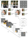
Design of stimuli and structure of a trial. (a) The procedure to generate probe patches. Each of the 9 patches were tagged with a location number 1–9 corresponding to their locations in the original image. (b) Summary of the congruence manipulation of the initial image and subsequent probe patches. The initial image is ‘congruent’ if it contains an object (i.e. headphone) which is congruent with the scene-gist (i.e. a girl listening to music). The initial image is ‘incongruent’ if it contains an object (i.e. doughnut) which is incongruent with the scene-gist. The probe object patch can be either ‘modified’ or ‘original’ with respect to the initial image (regardless of congruence of the initial image). (c) Example single-trial procedure of the experiment. At the beginning of a trial, a fixation cross appeared at the centre of the display for 500 ms. Then, either a congruent or incongruent initial image was presented for 133 ms. The image was masked by a sequence of 5 scrambled images, with each mask presented for 60 ms. After the mask images disappeared from the display, participants viewed and responded to each of the 20 probe patches (the 6 probe patches in Experiment 2). Each patch was presented for 133 ms and followed by 5 scrambled image masks of the same size as the patch. Participants had unlimited time to make a response on the response screen. (d) The response screen consists of 8 alternatives with 4 levels of confidence for both Yes and No options.

Figure 2.

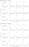
Mean percentages of responses (y-axis) as a function of decision (‘present’ = 1, ‘absent’ = −1) confidence (1–4) (x-axis) across participants in (i) Experiment 1 (top panels, in-laboratory, N = 15) and (ii) Experiment 2 (bottom panels, online, registered, N = 240). For each experiment, in each panel (a–l), values denoted by each colour line sum up to 1. Error bars represent standard error of the mean across subjects. Response proportion for (a–d) present + original patches (solid orange) and null patches (solid pink), (e–h) original (solid blue) and modified object probes (solid red) after the congruent initial images and (i–l) original (dotted blue) and modified (dotted red) object probes after the incongruent initial images. (a,e,i) Data pooled across eccentricities. The three right-hand columns ((b,f,j), (c,g,k) and (d,h,l)) represent the results with patches presented at eccentricity of 0, 6.5 and 9.2 dva for Experiment 1, and foveal, para-foveal, and peripheral for Experiment 2, respectively. We show * = p < 0.003 and ** = p < 0.0001 from t-tests comparing percentages of responses between present + original and null patches (a–d), and between original and modified patches (e–l), for a given D × C.

Figure 3.

Criterion-free analyses. Objective (top row) and subjective (bottom row) task performance in two types of image patch discrimination; present + original versus null patches (a and b), as well as original versus modified patches (c and d for congruent, and e and f for incongruent initial images) in Experiment 1 (blue, N = 15) and Experiment 2 (orange, registered, N = 240). Error bars represent standard error of the mean. Dotted black lines represent chance-level (0.5) performance.

Figure 4.

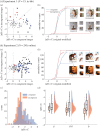
Image-based analysis of the effects of congruence of the initial images and object modification in Experiment 1 (i) and Experiment 2 (ii). Based on transformed D × C (tD × C), we define ΔtD × C as mean tD × C for the original probe − mean tD × C for the modified probe for each image pair. (i-a and ii-a) Scatterplots of ΔtD × C for the congruent (x-axis) and the incongruent (y-axis) initial images. Each dot represents the ΔtD × C for one image pair (N = 15 participants, with N = 3 to 12 for each image within the pair for Experiment 1 (i-a) and N = 30, with N = 15 each image for Experiment 2 (ii-a)). Four colors indicate the results of the statistical test (two-sample t-tests, p < 0.05, uncorrected). Grey: no significant difference between original and modified patch tD × C for both congruent and incongruent initial images. Blue: the difference between original and modified tD × C only significant for the congruent. Red: only significant for the incongruent. Black: significant for both. We also represented image pairs whose polarity of ΔtD × C are opposite (i.e. a significant interaction between patch response type (original/modified) and image congruence in two-way ANOVA) with dots with square outlines. There was no correlation between the congruent and the incongruent initial image in Experiment 1 (i-a) (R² = 0.03, p = 0.89) and a weak but significant correlation in Experiment 2 (ii-a) (R² = 0.10, p < 0.001). (i-b and ii-b) Cumulative histogram for ΔtD × C. The blue and red lines are the ΔtD × C for the congruent and incongruent initial images. Here we show two exemplar image pairs with their corresponding ΔtD × C (indicated by the source point of the arrows) as well as the original and modified probe patches. (ii-c) Histogram distribution of ΔtD × C in Experiment 2. (ii-d) Fitted distributions, boxplots and scatterplots of ΔtD × C against eccentricity levels (F, fovea; P-F, para-fovea; P, periphery) in Experiment 2.

Figure 5.

Size of the critical object explains the variance across image pairs and the congruence effects on ΔtD × C. (a) Sample image pair. (b,c) The estimation procedure for object sizes and Weibull scale parameter using the image pair in (a) as an example. To estimate the size of the critical object (b), we obtained the absolute difference in RGB for the two images, from which we detected the area of the object, thresholded as RGB difference = 10. We calculated the proportion of the area in the image as the size of the object. For estimating Weibull scale parameters (c), we filtered the original images to obtain the gradient magnitudes, and then plot the gradient magnitudes (black histograms) as the contrast distributions of the images. We fitted a Weibull distribution for each contrast distribution (orange line), and obtained the scale values β. For an extended description about the estimation of size and Weibull parameters, see electronic supplementary material, figures S3 and S4. (d) The relation between ΔtD × C and object size (log-scaled). Each dot represents an individual image pair. The colour lines represent the best fit regression lines estimated from LME analysis. Blue: congruent initial images. Red: incongruent initial images. (e) The relation between ΔtD × C and Weibull scale parameter values, in the same format as (d).

References

1. Laureys S. 2005. The neural correlate of (un) awareness: lessons from the vegetative state. Trends Cogn. Sci. 9, 556-559. (10.1016/j.tics.2005.10.010) - DOI - PubMed
1. Koch C, Massimini M, Boly M, Tononi G. 2016. Neural correlates of consciousness: progress and problems. Nat. Rev. Neurosci. 17, 307-321. (10.1038/nrn.2016.22) - DOI - PubMed
1. Dehaene S, Changeux JP. 2011. Experimental and theoretical approaches to conscious processing. Neuron 70, 200-227. (10.1016/j.neuron.2011.03.018) - DOI - PubMed
1. Rensink RA, O'regan JK, Clark JJ. 1997. To see or not to see: the need for attention to perceive changes in scenes. Psychol. Sci. 8, 368-373. (10.1111/j.1467-9280.1997.tb00427.x) - DOI
1. Simons DJ, Ambinder MS. 2005. Change blindness: theory and consequences. Curr. Dir. Psychol. Sci. 14, 44-48. (10.1111/j.0963-7214.2005.00332.x) - DOI
LinkOut - more resources