Supervised and Weakly Supervised Deep Learning for Segmentation and Counting of Cotton Bolls Using Proximal Imagery

Abstract

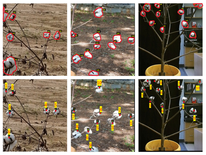
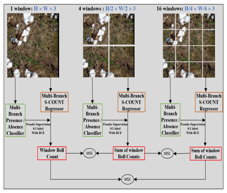
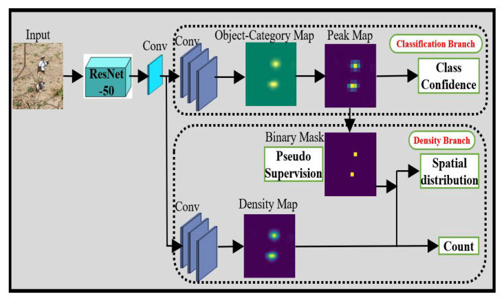
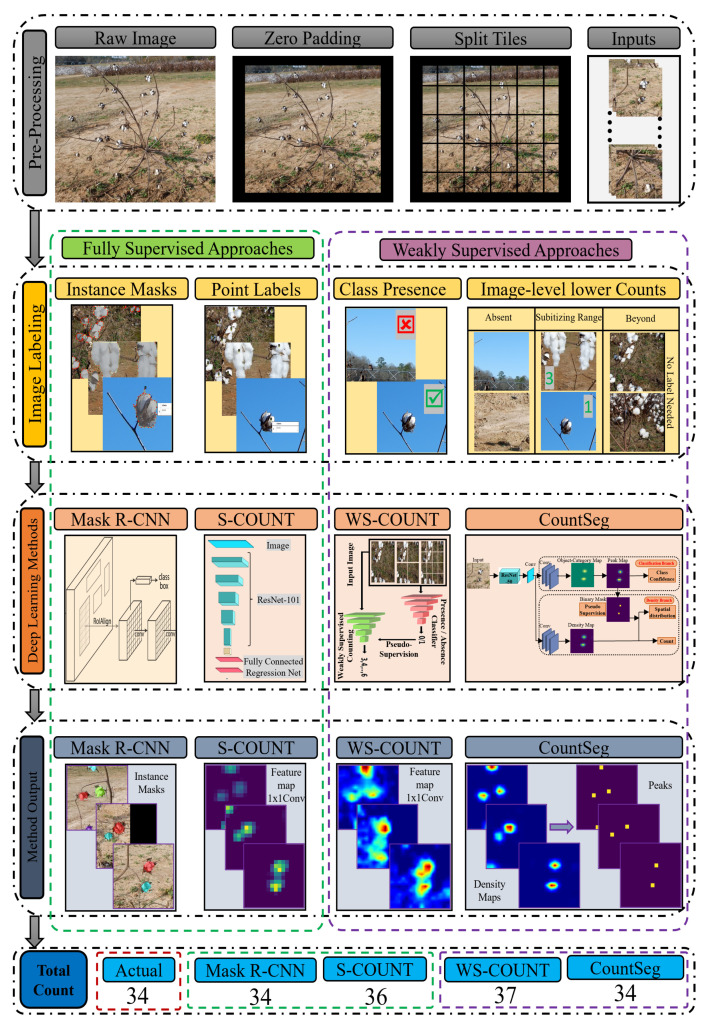
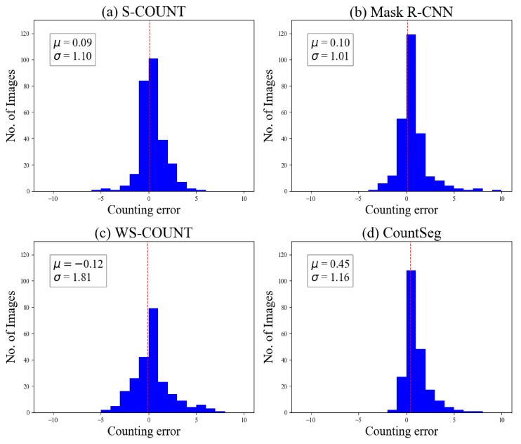
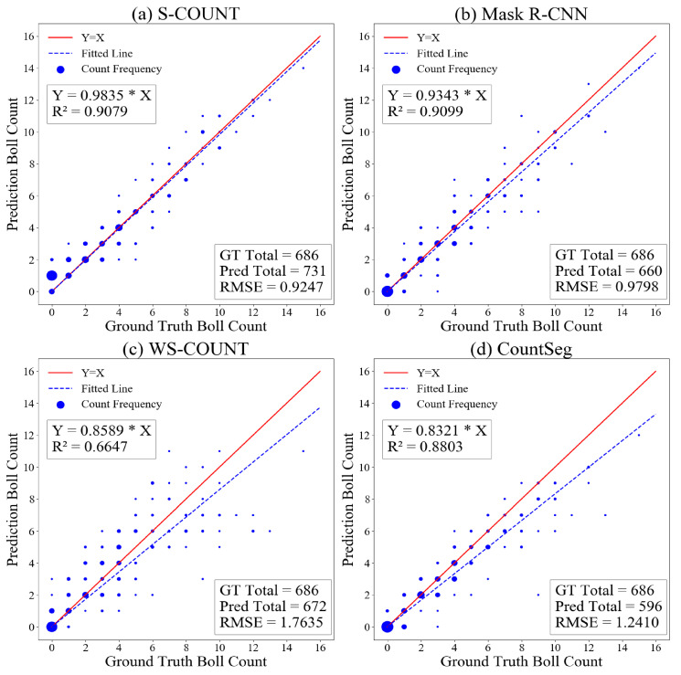
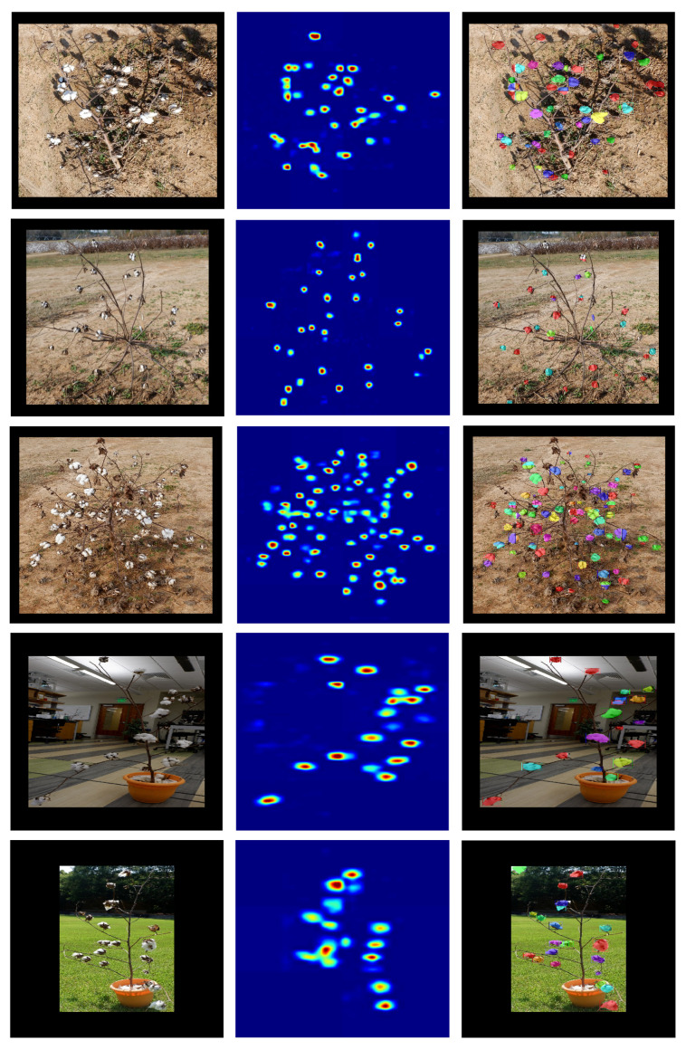
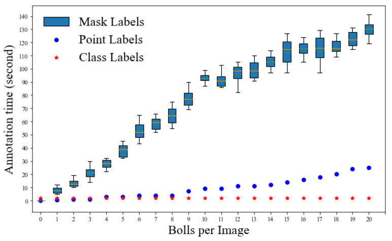
The total boll count from a plant is one of the most important phenotypic traits for cotton breeding and is also an important factor for growers to estimate the final yield. With the recent advances in deep learning, many supervised learning approaches have been implemented to perform phenotypic trait measurement from images for various crops, but few studies have been conducted to count cotton bolls from field images. Supervised learning models require a vast number of annotated images for training, which has become a bottleneck for machine learning model development. The goal of this study is to develop both fully supervised and weakly supervised deep learning models to segment and count cotton bolls from proximal imagery. A total of 290 RGB images of cotton plants from both potted (indoor and outdoor) and in-field settings were taken by consumer-grade cameras and the raw images were divided into 4350 image tiles for further model training and testing. Two supervised models (Mask R-CNN and S-Count) and two weakly supervised approaches (WS-Count and CountSeg) were compared in terms of boll count accuracy and annotation costs. The results revealed that the weakly supervised counting approaches performed well with RMSE values of 1.826 and 1.284 for WS-Count and CountSeg, respectively, whereas the fully supervised models achieve RMSE values of 1.181 and 1.175 for S-Count and Mask R-CNN, respectively, when the number of bolls in an image patch is less than 10. In terms of data annotation costs, the weakly supervised approaches were at least 10 times more cost efficient than the supervised approach for boll counting. In the future, the deep learning models developed in this study can be extended to other plant organs, such as main stalks, nodes, and primary and secondary branches. Both the supervised and weakly supervised deep learning models for boll counting with low-cost RGB images can be used by cotton breeders, physiologists, and growers alike to improve crop breeding and yield estimation.

Keywords: boll counting; cotton phenotyping; mask R-CNN; supervised learning; weakly supervised learning.

Figure 1

Annotation Types. Two main types of annotations were used in this study. The top row represents instance masks with class labels, whereas the bottom row represents point labels for the same image with the boll ID (the red numbers). The first column shows a sample tile from in-field plant image, whereas the second and third column show potted plants in outdoor and indoor conditions, respectively.

Figure 2

Schematic representation of WS-Count architecture. An image is divided into 4 windows and then further divided into 16 windows. A total of 21 images are passed to the main two networks that are responsible for boll counting. Presence Absence Classifier (PAC) detects the presence of boll in the patch and thus provides a weak supervision for the regression network, whereas the counting network (S-Count) estimates a boll count for that patch with the help of additional fully connected layers. The processing of 21 image patches in parallel makes the individual PAC and S-Count networks multi-branched (MB) and predicts unique output count for each of the 21 patches. The count predictions are kept in accordance with the classifier supervision and the total count loss is optimized through all the image levels.

Figure 3

CountSeg architecture for boll counting. The two branches, classification branch and density branch, are jointly trained using image-level lower-counts (ILC) supervision. The pseudo ground truth is generated by classification branch to supervise the output of density map with the help of spatial and global loss functions.

Figure 4

Overview of the boll counting workflow.The image tiles generated after pre-processing were labelled with point and mask labels. The classification labels ($✓\mathrm{and} \times$) and image-level boll counts (1, 2, 3…) were derived from point label counts. Two fully supervised and two weakly supervised counting methods were trained on the image tiles’ training set (Table 2). The intermediate and final stage output of each methods can be visualized by instance masks and feature maps that will be used to obtain final boll count. In this example, the raw image (top row) contains 34 cotton bolls which were predicted accurately by both the Mask R-CNN and CountSeg Methods.

Figure 5

Error histograms from median predictions given by each method. Error is computed as the difference between the ground truth count and median of predicted counts from five model variations.

Figure 6

Bubble plots and linear regression between ground truth and predicted boll counts. The total boll count from 200 validation images is shown to demonstrate counting capabilities of the method.

Figure 7

Comparison of CountSeg and Mask R-CNN. This shows the output from CountSeg density maps and prediction instance masks from Mask R-CNN for 5 held-out test samples (starting from the top row): Boll_008, Boll_022, Boll_041, Boll_116, Boll_127, respectively. It can be observed that even with lower supervision, CountSeg was able to retain the spatial contexts for most of the bolls.

Figure 8

Comparison of annotation time of three types of labels. The time taken for annotating an image tile was measured with respect to the boll count in that image tile. A sample set of 10 images per boll count was considered and the average times were reported for point labels whereas the box plots represent the range of time taken by mask labels for the same boll count.

References

1. FAOSTAT . FAOSTAT Statistical Database. FAO (Food and Agriculture Organization of the United Nations); Rome, Italy: 2019.
1. Pabuayon I.L.B., Kelly B.R., Mitchell-McCallister D., Coldren C.L., Ritchie G.L. Cotton boll distribution: A review. Agron. J. 2021;113:956–970. doi: 10.1002/agj2.20516. - DOI
1. Normanly J. High-Throughput Phenotyping in Plants: Methods and Protocols. Springer; Berlin/Heidelberg, Germany: 2012.
1. Pabuayon I.L.B., Yazhou S., Wenxuan G., Ritchie G.L. High-throughput phenotyping in cotton: A review. J. Cotton Res. 2019;2:1–9. doi: 10.1186/s42397-019-0035-0. - DOI
1. Uddin M.S., Bansal J.C. Computer Vision and Machine Learning in Agriculture. Springer; Berlin/Heidelberg, Germany: 2021.
LinkOut - more resources