Statistical power for cluster analysis

Abstract

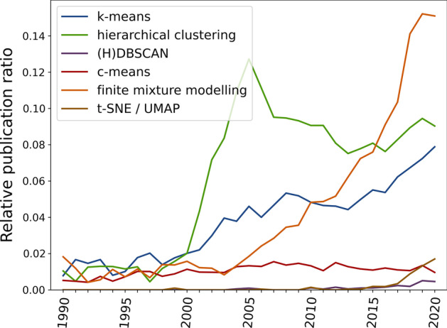
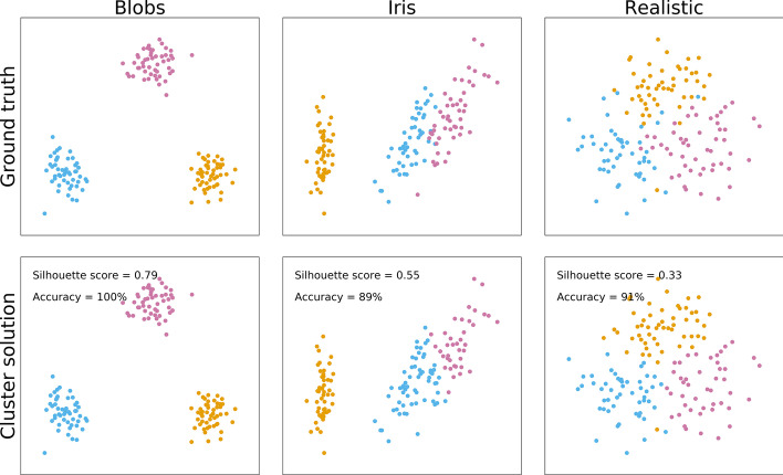
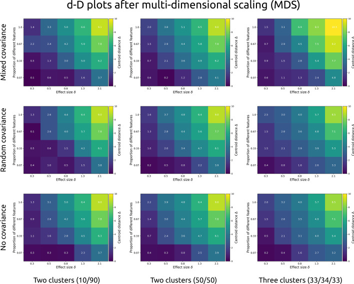
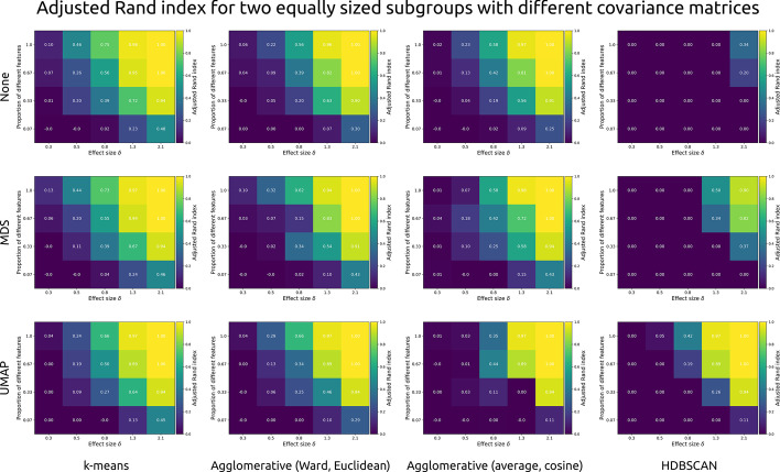
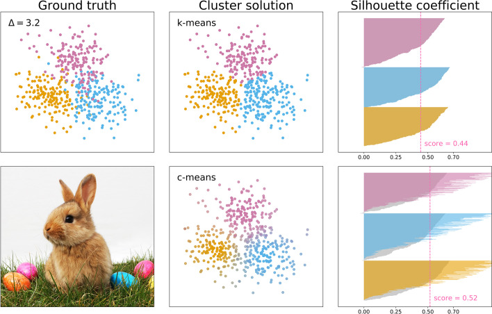
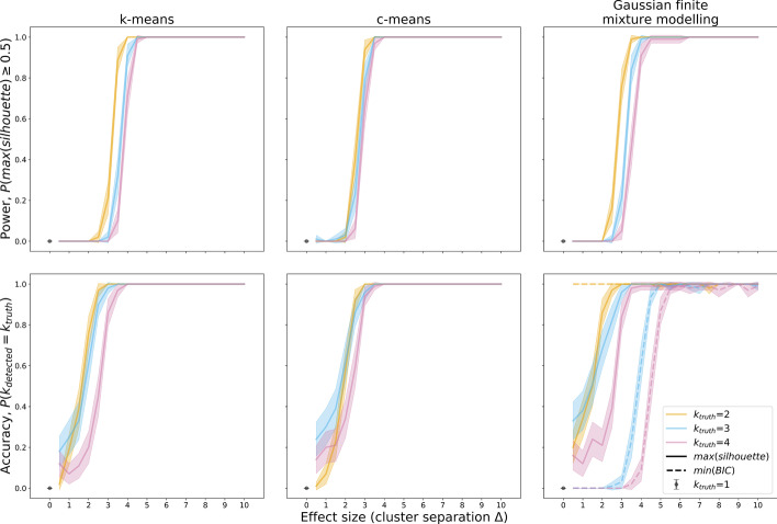
Background: Cluster algorithms are gaining in popularity in biomedical research due to their compelling ability to identify discrete subgroups in data, and their increasing accessibility in mainstream software. While guidelines exist for algorithm selection and outcome evaluation, there are no firmly established ways of computing a priori statistical power for cluster analysis. Here, we estimated power and classification accuracy for common analysis pipelines through simulation. We systematically varied subgroup size, number, separation (effect size), and covariance structure. We then subjected generated datasets to dimensionality reduction approaches (none, multi-dimensional scaling, or uniform manifold approximation and projection) and cluster algorithms (k-means, agglomerative hierarchical clustering with Ward or average linkage and Euclidean or cosine distance, HDBSCAN). Finally, we directly compared the statistical power of discrete (k-means), "fuzzy" (c-means), and finite mixture modelling approaches (which include latent class analysis and latent profile analysis).

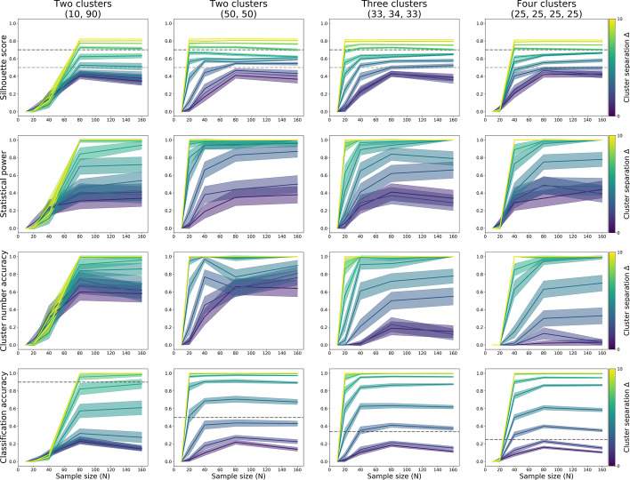
Results: We found that clustering outcomes were driven by large effect sizes or the accumulation of many smaller effects across features, and were mostly unaffected by differences in covariance structure. Sufficient statistical power was achieved with relatively small samples (N = 20 per subgroup), provided cluster separation is large (Δ = 4). Finally, we demonstrated that fuzzy clustering can provide a more parsimonious and powerful alternative for identifying separable multivariate normal distributions, particularly those with slightly lower centroid separation (Δ = 3).

Conclusions: Traditional intuitions about statistical power only partially apply to cluster analysis: increasing the number of participants above a sufficient sample size did not improve power, but effect size was crucial. Notably, for the popular dimensionality reduction and clustering algorithms tested here, power was only satisfactory for relatively large effect sizes (clear separation between subgroups). Fuzzy clustering provided higher power in multivariate normal distributions. Overall, we recommend that researchers (1) only apply cluster analysis when large subgroup separation is expected, (2) aim for sample sizes of N = 20 to N = 30 per expected subgroup, (3) use multi-dimensional scaling to improve cluster separation, and (4) use fuzzy clustering or mixture modelling approaches that are more powerful and more parsimonious with partially overlapping multivariate normal distributions.

Keywords: Cluster analysis; Covariance; Dimensionality reduction; Effect size; Latent class analysis; Latent profile analysis; Sample size; Simulation; Statistical power.

Fig. 1

The increase in publications indexed by PubMed that mention a keyword specific to cluster analyses relative to the number of publications that mention a traditional statistical test. Particularly sharp increases can be seen for finite mixture modelling (which includes latent class and latent profile analysis) and k-means. Illustration generated using Bibliobanana [17]. See “Methods” section for details on exact search terms

Fig. 2

This figure shows three datasets in the top row, each made up out of 150 observations that fall in three equally sized clusters. While the datasets are made up of 4 features, the plotted data is a two-dimensional projection through multi-dimensional scaling (MDS). The left column presents simulated “blobs” as they are commonly used in clustering tutorials, the middle column presents the popular Iris dataset, and the right presents more realistic multivariate normal distributions. The bottom row presents the outcome of k-means clustering, showing good classification accuracy for all datasets, but only reliable cluster detection (silhouette coefficient of 0.5 or over) for blobs and the Iris dataset, but not the more realistic scenario

Fig. 3

Each cell presents the cluster centroid separation Δ (brighter colours indicate stronger separation) after multi-dimensional scaling (MDS) was applied to simulated data of 1000 observations and 15 features. Separation is shown as a function of within-feature effect size (Cohen’s d, x-axis), and the proportion of features that were different between clusters. Each row shows a different covariance structure: “mixed” indicates subgroups with different covariance structures, “random” with the same random covariance structure between all groups, and “no” for no correlation between any of the features). Each column shows a different type of population: with unequal (10 and 90%) subgroups, with two equally sized subgroups, and with three equally sized subgroups

Fig. 4

Each cell presents the cluster centroid separation Δ (brighter colours indicate stronger separation) after uniform manifold approximation and projection (UMAP) was applied to simulated data of 1000 observations and 15 features. Separation is shown as a function of within-feature effect size (Cohen’s d, x-axis), and the proportion of features that were different between clusters. Each row shows a different covariance structure: “mixed” indicates subgroups with different covariance structures, “random” with the same random covariance structure between all groups, and “no” for no correlation between any of the features). Each column shows a different type of population: with unequal (10 and 90%) subgroups, with two equally sized subgroups, and with three equally sized subgroups

Fig. 5

Each cell shows the adjusted Rand index (brighter colours indicate better classification) as a function of within-feature effect size (Cohen’s d), and the proportion of features that differed between two simulated clusters with different covariance structures (3-factor and 4-factor). Each row presents a different dimensionality reduction approach: None, multi-dimensional scaling (MDS), or uniform manifold approximation and projection (UMAP). Each column presents a different type of clustering algorithm: k-means, agglomerative (hierarchical) clustering with Ward linkage and Euclidean distance, agglomerative clustering with average linkage and cosine distance, and HDBSCAN

Fig. 6

Each cell shows the silhouette coefficient (brighter colours indicate stronger detected clustering, with a threshold set at 0.5) as a function of within-feature effect size (Cohen’s d), and the proportion of features that differed between two simulated clusters with different covariance structures (3-factor and 4-factor). Each row presents a different dimensionality reduction approach: None, multi-dimensional scaling (MDS), or uniform manifold approximation and projection (UMAP). Each column presents a different type of clustering algorithm: k-means, agglomerative (hierarchical) clustering with Ward linkage and Euclidean distance, agglomerative clustering with average linkage and cosine distance, and HDBSCAN

Fig. 7

Each dot represents a simulated dataset of 1000 observations and 15 features, each with different within-feature effect size, proportion of different features between clusters, covariance structure, and number of clusters. The x-axis represents the separation between subgroups in the population that datasets were simulated from, and the y-axis represents the separation in the simulated dataset after no dimensionality reduction (green), multi-dimensional scaling (MDS, blue), or uniform manifold approximation and projection (UMAP, purple). The dotted line indicates no difference between population and sample; values above the dotted line have had their separation increased, and it was decreased for those below the line

Fig. 8

K-means silhouette scores (top row), proportion of correctly identified clustering (second row), proportion of correctly identified number of clusters (third row), and the proportion of observations correctly assigned to their subgroup, each computed through 100 iterations of simulation. Datasets of varying sample size (x-axis) and two features were sampled from populations with equidistant subgroups that each had the same 3-factor covariance structure. The simulated populations were made up of two unequally sized (10 and 90%) subgroups (left column); or two, three, or four equally sized subgroups (second, third, and fourth column, respectively)

Fig. 9

HDBSCAN silhouette scores (top row), proportion of correctly identified clustering (second row), proportion of correctly identified number of clusters (third row), and the proportion of observations correctly assigned to their subgroup, each computed through 100 iterations of simulation. Datasets of varying sample size (x-axis) and two features were sampled from populations with equidistant subgroups that each had the same 3-factor covariance structure. The simulated populations were made up of two unequally sized (10 and 90%) subgroups (left column); or two, three, or four equally sized subgroups (second, third, and fourth column, respectively)

Fig. 10

C-means silhouette scores (top row), proportion of correctly identified clustering (second row), proportion of correctly identified number of clusters (third row), and the proportion of observations correctly assigned to their subgroup, each computed through 100 iterations of simulation. Datasets of varying sample size (x-axis) and two features were sampled from populations with equidistant subgroups that each had the same 3-factor covariance structure. The simulated populations were made up of two unequally sized (10 and 90%) subgroups (left column); or two, three, or four equally sized subgroups (second, third, and fourth column, respectively)

Fig. 11

Clustering outcomes of discrete k-means clustering (top row) and fuzzy c-means clustering (bottom row). The top-left panel shows the ground truth, a sample (N = 600) from a simulated population made up of three equally sized and equidistant subgroups. The middle column shows the assignment of observations to clusters, and the right column shows the corresponding silhouette coefficients. The shading in the bottom silhouette plot indicates the discrete clustering silhouette coefficients, and the coloured bars indicate a transformation equivalent to that performed to compute the fuzzy silhouette score. The bottom-left shows a bunny (also fuzzy) amid contained and well-separated ellipsoidal clusters (photo by Tim Reckmann, licensed CC-BY 2.0)

Fig. 12

Traditional (top row), fuzzy (middle row and bottom row) silhouette scores, respectively computed after clustering through k-means, c-means, and Gaussian finite mixture modelling. Each line presents the mean and 95% confidence interval obtained over 100 iterations of sampling (N = 120, two uncorrelated features) from populations with no subgroups (left column), two subgroups (second column), three subgroups (third column), or four subgroups (right column) that were equidistant and of equal size. The same dataset in each iteration was subjected to k-means, c-means, and Gaussian mixture modelling. Estimates were obtained for different centroid separation values (Δ = 1 to 10, in steps of 0.5; brighter colours indicate stronger separation). All simulation results are plotted, and power (proportion of iterations that found k > 1) and accuracy (proportion of iterations that found the true number of clusters) are annotated for centroid separations Δ = 2 to 4 (see Fig. 13 for power and accuracy as a function of centroid separation)

Fig. 13

Power (top row) and cluster number accuracy (bottom row) for k-means (left column), c-means (middle column), and Gaussian mixture modelling (right column). Power was computed as the proportion of simulations in which the silhouette score was equal to or exceeded 0.5, the threshold for subgroups being present in the data. Cluster number accuracy was computed as the proportion of simulations in which the highest silhouette coefficient (solid lines) or the lowest Bayesian Information Criterion (dashed line, only applicable in Gaussian mixture modelling) was associated with the true simulated number of clusters. For each ground truth k = 1 to k = 4, 100 simulation iterations were run. In each iteration, all three methods were employed on the same data, and all methods were run for guesses k = 2 to k = 7

References

1. Handelsman DJ, Teede HJ, Desai R, Norman RJ, Moran LJ. Performance of mass spectrometry steroid profiling for diagnosis of polycystic ovary syndrome. Hum Reprod. 2017;32(2):418–422. doi: 10.1093/humrep/dew328. - DOI - PubMed
1. Pedregosa F, Varoquaux G, Gramfort A, Michel V, Thirion B, Grisel O, et al. Scikit-learn: machine learning in Python. J Mach Learn Res. 2011;12:2825–2830.
1. Hennig C. fpc. 2020. Available from https://cran.r-project.org/web/packages/fpc/index.html.
1. Anjana RM, Baskar V, Nair ATN, Jebarani S, Siddiqui MK, Pradeepa R, et al. Novel subgroups of type 2 diabetes and their association with microvascular outcomes in an Asian Indian population: a data-driven cluster analysis: the INSPIRED study. BMJ Open Diabetes Res Care. 2020;8(1):e001506. doi: 10.1136/bmjdrc-2020-001506. - DOI - PMC - PubMed
1. Tao R, Yu X, Lu J, Shen Y, Lu W, Zhu W, et al. Multilevel clustering approach driven by continuous glucose monitoring data for further classification of type 2 diabetes. BMJ Open Diabetes Res Care. 2021;9(1):e001869. doi: 10.1136/bmjdrc-2020-001869. - DOI - PMC - PubMed
LinkOut - more resources