The normative modeling framework for computational psychiatry

Abstract

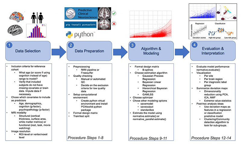
Normative modeling is an emerging and innovative framework for mapping individual differences at the level of a single subject or observation in relation to a reference model. It involves charting centiles of variation across a population in terms of mappings between biology and behavior, which can then be used to make statistical inferences at the level of the individual. The fields of computational psychiatry and clinical neuroscience have been slow to transition away from patient versus 'healthy' control analytic approaches, probably owing to a lack of tools designed to properly model biological heterogeneity of mental disorders. Normative modeling provides a solution to address this issue and moves analysis away from case-control comparisons that rely on potentially noisy clinical labels. Here we define a standardized protocol to guide users through, from start to finish, normative modeling analysis using the Predictive Clinical Neuroscience toolkit (PCNtoolkit). We describe the input data selection process, provide intuition behind the various modeling choices and conclude by demonstrating several examples of downstream analyses that the normative model may facilitate, such as stratification of high-risk individuals, subtyping and behavioral predictive modeling. The protocol takes ~1-3 h to complete.

Figure 1. Conceptual Overview of Normative Modeling.

A) Classical example of normative modeling: the use of height and weight growth charting in pediatrics. B) Case-control models (left) theoretically make assumptions that there is a boundary that can separate groups and that there is within-group homogeneity. In reality (right), there is nested variation across controls and patient groups and within-group heterogeneity, resulting in unclear separation boundaries. Normative modeling is well equipped to handle this reality. C) An example application of normative modeling in computational psychiatry using neuroimaging data. Mean cortical thickness (y-axis) is predicted from age (x-axis) using a training set consisting of multi-site structural MRI from neurotypical controls and a test set consisting of neurotypical controls and patient groups. Every dot indicates the deviation score for a single individual from normal development. D) Regression model equation and design matrix setup for the model shown in panel C.

Figure 2. Practical Overview of Normative Modeling Framework.

The workflow consists of four stages: data selection, data preparation, algorithm & modeling, and evaluation & interpretation, which are visualized by the numbered shaded blue boxes. The steps involved at each of these stages are summarized in the box below and highlighted in the images above.

Figure 3. Overview of Resources for Running a Normative Modeling Analysis.

A) Detailed documentation, including installation instructions, input/output descriptions of all classes and functions implemented in the python package, tutorials for all algorithms, frequently asked questions, a glossary explaining acronyms and other jargon, references to existing normative modeling literature, and a citation guide, is available online. B) Example of the documentation showing the required input, expected output of the main function used in the pcntoolkit software, the estimate function. C) All of the code and data used in this protocol is available to run in the cloud via Google Colab. Additional tutorials (shown under the tutorials header in panel A) are also available to run in Google Colab.

Figure 4. Visualization of Normative Model Evaluation Metrics.

A) A ridge plot showing the distribution across all brain regions of the standardized mean squared error (SMSE), an evaluation metric that represents accuracy, visualized for each site in the test set. Visualizing for each test site can help identify if there are sites where the model is performing poorly. Ideally, the distribution will be Gaussian and should look similar across all sites. Small shifts in the mean across sites is to be expected and is acceptable. B) Explained variance is shown for cortical thickness of every brain region in the Destrieux parcellation) and volume of subcortical regions. Visualizing the evaluation metrics in brain space helps to identify patterns and see the big picture. C) The number of extreme deviations (both positive and negative) are counted for each individual in the test set, group ID is used to plot the distribution of the extreme deviation count for each group. A statistical test can be done on the count to determine if there is a significant difference between groups. Testing group differences in the count of deviations does not require there to be spatial overlap of the deviations within the group (i.e., this test can account for within-group heterogeneity of deviations). D) The normative trajectory for an example brain region (lateral ventricle) showing age (x-axis) versus the predicted volume (y-axis). The centiles of variation are shown by the lines and shaded confidence intervals. Each subject in the test set is plotted as a single point. E-F) Extreme deviations, separated into positive (E) and negative (F), are summarized for each group. For each brain region, the number of subjects with an extreme deviation in that region is counted, then divided by the group sample size, to show the percent of subjects with an extreme deviation. These visualizations demonstrate the benefit of normative modeling as there is within group heterogeneity that other methods (i.e., case-control group difference testing) are not equipped to handle. Abbreviations: HC = Controls, MDD=Major Depressive Disorder, SZ=Schizophrenia, SAD=Social Anxiety Disorder, EP=Early Psychosis.

References

1. Wang D, et al. Parcellating cortical functional networks in individuals. Nat Neurosci. 2015;18:1853–1860. - PMC - PubMed
1. Finn ES, Constable RT. Individual variation in functional brain connectivity: implications for personalized approaches to psychiatric disease. Dialogues Clin Neurosci. 2016;18:277–287. - PMC - PubMed
1. Braga RM, Buckner RL. Parallel Interdigitated Distributed Networks within the Individual Estimated by Intrinsic Functional Connectivity. Neuron. 2017;95:457–471.:e5. - PMC - PubMed
1. Poldrack RA. Precision Neuroscience: Dense Sampling of Individual Brains. Neuron. 2017;95:727–729. - PubMed
1. Vanderwal T, et al. Individual differences in functional connectivity during naturalistic viewing conditions. NeuroImage. 2017;157:521–530. - PubMed
Publication types