The emergence of a collective sensory response threshold in ant colonies

Abstract

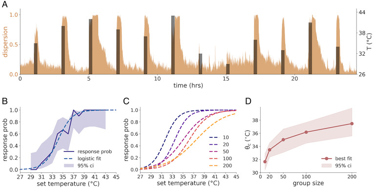
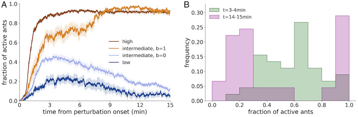
SignificanceIn this study, we ask how ant colonies integrate information about the external environment with internal state parameters to produce adaptive, system-level responses. First, we show that colonies collectively evacuate the nest when the ground temperature becomes too warm. The threshold temperature for this response is a function of colony size, with larger colonies evacuating the nest at higher temperatures. The underlying dynamics can thus be interpreted as a decision-making process that takes both temperature (external environment) and colony size (internal state) into account. Using mathematical modeling, we show that these dynamics can emerge from a balance between local excitatory and global inhibitory forces acting between the ants. Our findings in ants parallel other complex biological systems like neural circuits.

Keywords: Ooceraea biroi; collective behavior; decision making; distributed computing; social insects.

Fig. 1.

The response of an ant colony to a step temperature perturbation. (A) A snapshot from a raw experimental video, showing a colony of 36 ants on a temperature-controlled plaster of Paris arena (Materials and Methods and SI Appendix, Figs. S1 and S2). Each of the ants is marked with a unique combination of color tags to allow for individual behavioral tracking. The arena is confined by a black metal frame heated to 50 °C (SI Appendix, Fig. S2). The ants form a nest (red square at the bottom and Inset at top right), with a few scout ants exploring the arena (top red square and Inset at top left). The light brown objects in the arena are food items. (B–I) Snapshots depicting the typical dynamics of the response of a colony to a strong temperature perturbation. Images are processed by removing the background for visual clarity. (B) Baseline state. Before the onset of the perturbation, most ants reside in the nest, with few scout ants exploring the arena. (C) Excitement. Following the onset of the perturbation, the ants first respond by increasing their activity level around the nest. (D) Evacuation onset. After a delay that lasts up to a few minutes, the ants suddenly begin to leave the nest in a well-defined direction. (E) Full evacuation. The colony forms a well-organized evacuation column. (F) Stable evacuation. (G) Disordered perturbed state. In some cases, especially under high-temperature perturbations, the organized evacuation column breaks, and the colony enters into a high-activity, swarm-like state, where the movements of the ants are only weakly correlated. (H) Relaxation. Following the return of the temperature to baseline, the ants slowly relax and begin to reform the nest, possibly in a different location. The relaxation process can take up to 1 h to complete. (I) New baseline. The colony has fully returned to its baseline relaxed state.

Fig. 2.

Ants respond collectively to temperature perturbations. (A) Measures of individual responses. We define a circle of radius R = 15 mm around the location of the nest. A schematic drawing of the trajectories of two ants is depicted in green and pink. For each ant, we record the binary response ($b$), the response direction ($\alpha$), and the response latency ($\tau$) as its first crossing of that circle for a duration longer than 30 s, as explained in the text and Materials and Methods. (B) Histograms of the average binary response across ants. Each histogram is constructed from one colony subjected to a sequence of 24 perturbations of 33 °C. (C) Pairwise correlations between the binary responses of ants in B, compared to correlations in shuffled responses. Shuffled responses are generated by shuffling the binary responses of each ant to all the perturbations independently of other ants in its colony, therefore eliminating any correlation. The real distribution is composed of 1,890 correlation values, produced from the responses of 108 ants from three colonies. The null distribution is composed of 189,000 correlation values, produced from 100 independent shuffles of the responses. (D) Scatter plot depicting the distributions of individual response latencies, from three colonies subjected to a sequence of 24 perturbations of 40 °C. Each column represents the responses of ants from a single colony to one perturbation. The events are sorted first by colony and then by the average individual response latency in each event. (E) Pairwise correlations between the response latencies of ants in D compared to a null distribution generated in the same way as in C. (F and G) Plots as in D and E, but for the individual response directions. Note that the response direction measure is cyclic, but because the per-event distribution (one column in F) is narrowly distributed around the average colony direction, this does not have a significant effect on the analysis.

Fig. 3.

The collective threshold depends on group size. (A) A trace from a 24-h-long perturbation protocol using a colony of 36 tagged ants. Perturbations are 15 min long and separated by intervals of 2 h. The set temperature is shown in black. The dispersion of the colony (defined as the fraction of ants outside the nest circle) is shown in brown. The interval allows the colony to relax back to baseline before the next perturbation. (B) The probability of a “full response” (defined as at least 90% of the ants being outside the nest at the same time for at least 30 s at some point during the perturbation; solid line) as a function of the perturbation temperature. The shaded band represents the 95% CI of probability (computed using asymptotic normal approximation for binary coefficient estimation). The dashed line represents a logistic regression fit of the response curve. Experimental colonies consisted of 36 tagged ants. (C) Fitted logistic regression curves as in B for different colony sizes, showing an upward shift in the response curve. (D) The collective threshold parameter ${\theta }_c,$ estimated by logistic regression, as a function of colony size. The shaded band represents the 95% CI, estimated using the bootstrap method with 1,000 sample repetitions (Materials and Methods).

Fig. 4.

The response dynamics are characterized by distinct timescales and social feedback. (A) The evolution in time of the colony state variable (the fraction of active ants) following a temperature change. Single-trial response curves from all experiments with 36 ants were averaged according to temperature and collective response condition. The dark brown curve represents the average response for high-temperature perturbations, for which the response probability was larger than 0.9. Events without a full response (b = 0) were excluded. The light brown curve represents the average response for intermediate-temperature perturbations (response probability between 0.1 and 0.9) in which the colony responded (b = 1). Responses in the same temperature range, but in which the colony did not respond (b = 0), are depicted by the light blue curve. Finally, the dark blue curve represents the average response for low-temperature perturbations [response probability smaller than 0.1; events with positive response (b = 1) were excluded]. (B) Histograms showing distributions of single-trial colony activity states for the intermediate-temperature range where the response probability is between 0.1 and 0.9, at two time points along the response curve. The green histogram shows the distribution for the interval between 3 and 4 min following perturbation onset, roughly corresponding to a time window in which the effect of the faster process has been exhausted, while the effect of the slower process is not yet apparent. Each datapoint in the histogram is the median value of a single perturbation event in that segment. The pink histogram shows the distribution for the interval between 14 and 15 min, when both transient dynamics of the response have run their course.

Fig. 5.

The emergence of the collective threshold can be modeled with two opposing forces. (A) An illustration of the model’s two-stage dynamics. In the first stage, the ants respond independently according to their individual response thresholds. As a result, a subset of ants becomes active. In the second stage, the interactions between the ants result in the colony being either fully active or fully inactive. (B) The logistic activation function of the individual ant. The ant is either active or inactive in a probabilistic manner depending on an integrated input parameter $h_i.$ The $\beta$ parameter controls the width of the ambiguous response region. (C) The individual response thresholds ${\theta }_i$ are sampled from a normal distribution of mean ${\theta }_m$ and width ${\theta }_{SD}.$ The collective threshold ${\theta }_c$ is the temperature for which the cumulative probability equals $m_c.$ (D) Simulation of the collective threshold, showing the response probability as a function of temperature, averaged over 100 simulation runs. For each run, a new set of individual thresholds is sampled. See Materials and Methods for full details on the simulation parameters. (E) The collective threshold as a function of group size for the basic model (gray circles) and the asymmetric model (purple circles). The interaction parameters $J^p$ and $J^r$ were chosen to have the same collective threshold at $N=50$ and to approximately replicate the range of thresholds observed in the experiment. (F) An illustration of possible ant interaction mechanisms. (Top) Global, pheromone-based interaction, in which ants in a given state contribute (black arrows) to the total concentration of pheromone in the environment (blue circle), which is then perceived by all ants (blue arrows). (Bottom) Local, contact-based interaction, in which ants in a given state affect only the behavior of nearby ants (red arrows).

References

1. Branco T., Redgrave P., The neural basis of escape behavior in vertebrates. Annu. Rev. Neurosci. 43, 417–439 (2020). - PubMed
1. Card G. M., Escape behaviors in insects. Curr. Opin. Neurobiol. 22, 180–186 (2012). - PubMed
1. Ter Hofstede H. M., Schöneich S., Robillard T., Hedwig B., Evolution of a communication system by sensory exploitation of startle behavior. Curr. Biol. 25, 3245–3252 (2015). - PubMed
1. Davidson J. D., El Hady A., Foraging as an evidence accumulation process. PLOS Comput. Biol. 15, e1007060 (2019). - PMC - PubMed
1. Levy S., Bargmann C. I., An adaptive-threshold mechanism for odor sensation and animal navigation. Neuron 105, 534–548.e13 (2020). - PubMed
Publication types
LinkOut - more resources