Ambient Air Pollution and Socioeconomic Status in China

Abstract

Background: Air pollution disparities by socioeconomic status (SES) are well documented for the United States, with most literature indicating an inverse relationship (i.e., higher concentrations for lower-SES populations). Few studies exist for China, a country accounting for 26% of global premature deaths from ambient air pollution.

Objective: Our objective was to test the relationship between ambient air pollution exposures and SES in China.

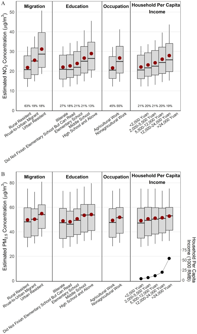
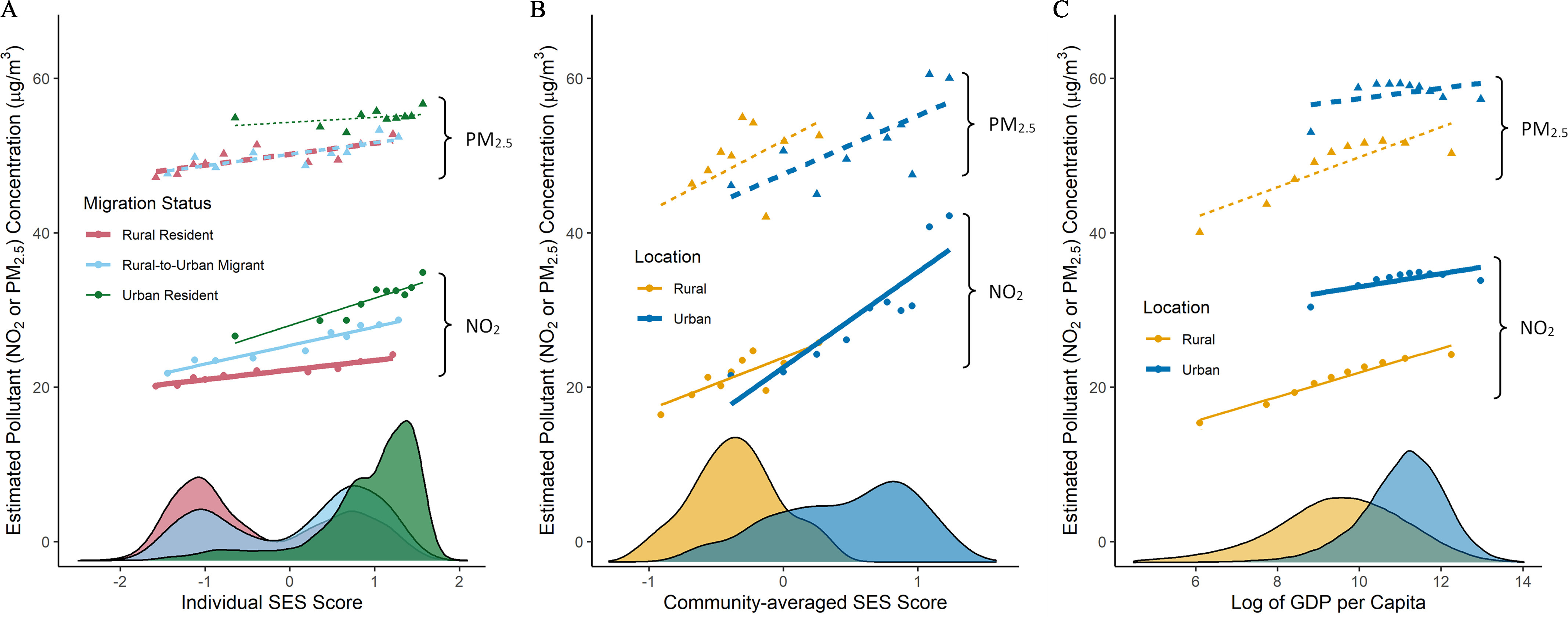
Methods: We combined estimated year 2015 annual-average ambient levels of nitrogen dioxide (${\mathrm{NO}}_2$) and fine particulate matter [PM $\le 2.5\mu m$ in aerodynamic diameter (${\mathrm{PM}}_{2.5}$)] with national demographic information. Pollution estimates were derived from a national empirical model for China at $1\text{-km}$ spatial resolution; demographic estimates were derived from national gridded gross national product (GDP) per capita at $1\text{-km}$ resolution, and (separately) a national representative sample of 21,095 individuals from the China Health and Retirement Longitudinal Study (CHARLS) 2015 cohort. Our use of global data on population density and cohort data on where people live helped avoid the spatial imprecision found in publicly available census data for China. We quantified air pollution disparities among individual's rural-to-urban migration status; SES factors (education, occupation, and income); and minority status. We compared results using three approaches to SES measurement: individual SES score, community-averaged SES score, and gridded GDP per capita.

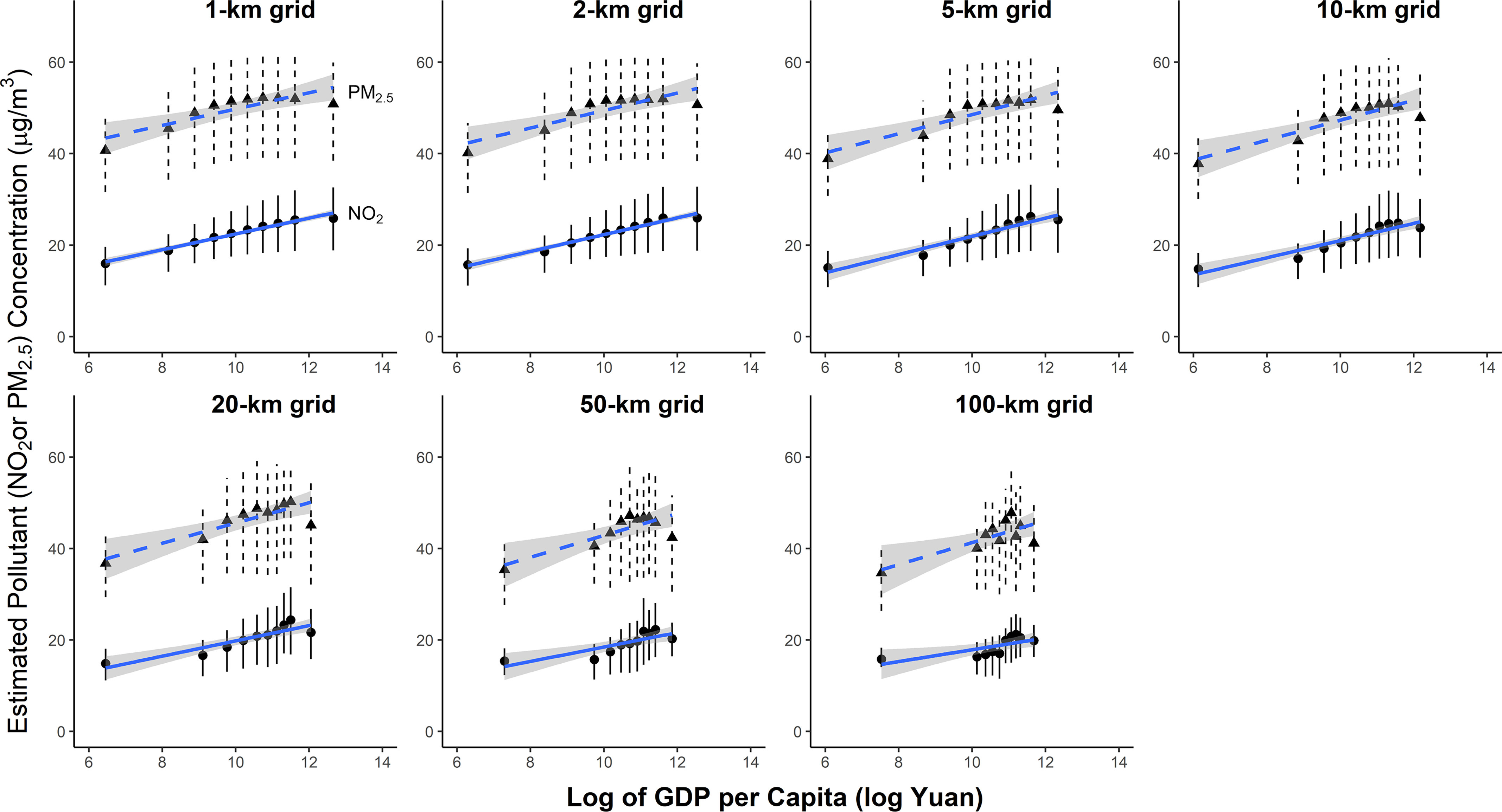
Results: Ambient ${\mathrm{NO}}_2$ and ${\mathrm{PM}}_{2.5}$ levels were higher for higher-SES populations than for lower-SES population, higher for long-standing urban residents than for rural-to-urban migrant populations, and higher for the majority ethnic group (Han) than for the average across nine minority groups. For the three SES measurements (individual SES score, community-averaged SES score, gridded GDP per capita), a 1-interquartile range higher SES corresponded to higher concentrations of $6-9{\mu g/m}^3$ ${\mathrm{NO}}_2$ and $3-6{\mu g/m}^3$ ${\mathrm{PM}}_{2.5}$; average concentrations for the highest and lowest 20th percentile of SES differed by 41-89% for ${\mathrm{NO}}_2$ and 12-25% for ${\mathrm{PM}}_{2.5}$. This pattern held in rural and urban locations, across geographic regions, across a wide range of spatial resolution, and for modeled vs. measured pollution concentrations.

Conclusions: Multiple analyses here reveal that in China, ambient ${\mathrm{NO}}_2$ and ${\mathrm{PM}}_{2.5}$ concentrations are higher for high-SES than for low-SES individuals; these results are robust to multiple sensitivity analyses. Our findings are consistent with the idea that in China's current industrialization and urbanization stage, economic development is correlated with both SES and air pollution. To our knowledge, our study provides the most comprehensive picture to date of ambient air pollution disparities in China; the results differ dramatically from results and from theories to explain conditions in the United States. https://doi.org/10.1289/EHP9872.

Figure 1.

Estimated ambient (A) ${\mathrm{NO}}_2$ and (B) ${\mathrm{PM}}_{2.5}$ concentration by individual’s rural-to-urban migration status, education, occupation, and income quintile. Box and whiskers indicate the 10th, 25th, 50th, 75th, and 90th percentiles and the mean (red circle). Income levels are displayed in the lower right of (B). The percentage numbers of individuals in each subgroup are annotated at the bottom of (A). Note: ${\mathrm{NO}}_2$, nitrogen dioxide; ${\mathrm{PM}}_{2.5}$, fine particulate matter, RMB, Renminbi.

Figure 2.

Relationship between SES and ambient ${\mathrm{NO}}_2$ and ${\mathrm{PM}}_{2.5}$ concentrations, based on (A) individual data, (B) areal data derived by aggregating the individual data to the community-level, and (C) areal data derived from national gridded GDP and world population density data sets. Data are plotted by urban–rural status, reflecting available data for individual data (A), three groups (rural resident, urban resident, and rural-to-urban migrant); for areal data (B,C), two groups (rural, urban). SES values reflect available data: (A) individual SES, (B) community-averaged SES, and (C) GDP per capita. Each plotted point represents the mean pollution concentration for 10% of the subsample. For example, in (A), the left-most red point represents the 10% of the rural residents with the lowest standardized SES score, and the right-most blue point represents the 10% of the rural-to-urban migrants with the highest standardized SES score. Plots also display best-fit lines and kernel densities. All of the best-fit lines have a positive slope {$p<0.002$ in all cases, except one [${\mathrm{PM}}_{2.5}$ for urban residents in (A); $p=0.48$]; for ${\mathrm{NO}}_2$ in (B) and all conditions in (C), $p<1\times {10}^{-6}$}, indicating that in all cases considered, higher SES is correlated with higher concentrations of ambient air pollution. Note: GDP, gross national product; ${\mathrm{NO}}_2$, nitrogen dioxide; ${\mathrm{PM}}_{2.5}$, fine particulate matter; SES, socioeconomic status.

Figure 3.

Relationship between pollution concentration and log GDP per capita, by grid cell size. Each point shows the mean log GDP per capita and mean pollution concentration of every 10% of population; each segment shows the IQR of pollution concentration. Best-fit lines by pollutant are shown in each plot. Note: GDP, gross national product; IQR, interquartile range; ${\mathrm{NO}}_2$, nitrogen dioxide; ${\mathrm{PM}}_{2.5}$, fine particulate matter.

References

1. Afridi F, Li SX, Ren Y. 2015. Social identity and inequality: the impact of China’s hukou system. J Public Econ 123:17–29, 10.1016/j.jpubeco.2014.12.011. - DOI
1. Baccarelli AA, Zheng Y, Zhang X, Chang D, Liu L, Wolf KR, et al. 2014. Air pollution exposure and lung function in highly exposed subjects in Beijing, China: a repeated-measure study. Part Fibre Toxicol 11:51, PMID: , 10.1186/s12989-014-0051-7. - DOI - PMC - PubMed
1. Baumgartner J, Schauer JJ, Ezzati M, Lu L, Cheng C, Patz J, et al. 2011. Patterns and predictors of personal exposure to indoor air pollution from biomass combustion among women and children in rural China. Indoor Air 21(6):479–488, PMID: , 10.1111/j.1600-0668.2011.00730.x. - DOI - PubMed
1. Beelen R, Raaschou-Nielsen O, Stafoggia M, Andersen ZJ, Weinmayr G, Hoffmann B, et al. 2014. Effects of long-term exposure to air pollution on natural-cause mortality: an analysis of 22 European cohorts within the multicentre ESCAPE project. Lancet 383(9919):785–795, PMID: , 10.1016/S0140-6736(13)62158-3. - DOI - PubMed
1. Beijing City Lab. 2014. Figure 1. Data 22: Urban areas of China in 2012 (by various methods). http://www.beijingcitylab.com [accessed 8 October 2020].
Publication types