Graph pangenome captures missing heritability and empowers tomato breeding

Abstract

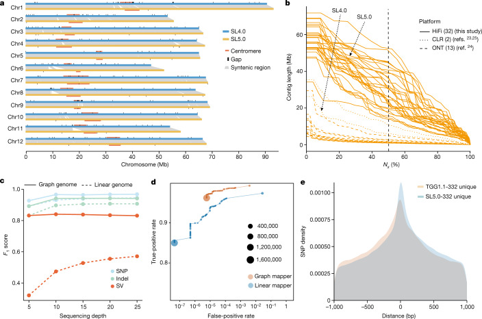
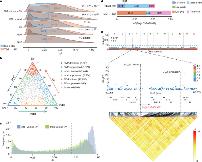
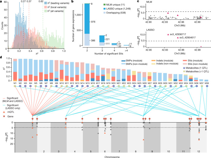
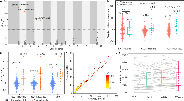
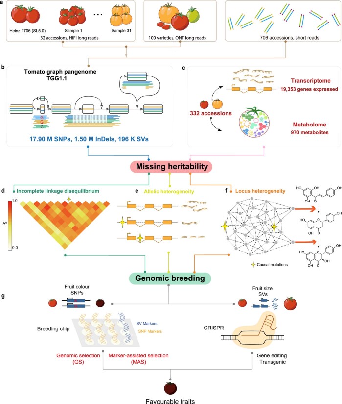
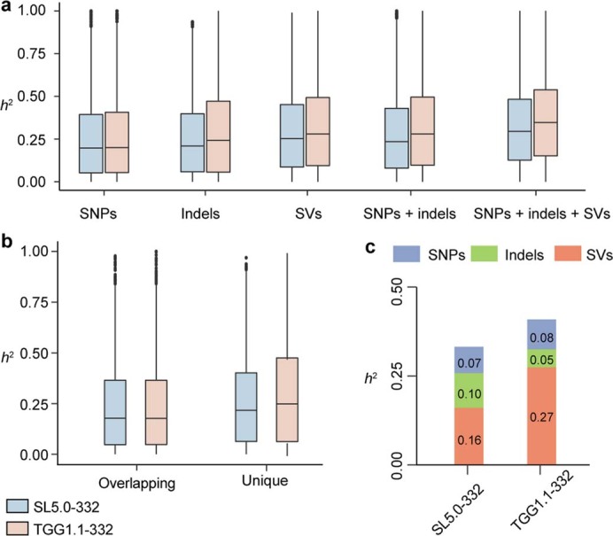
Missing heritability in genome-wide association studies defines a major problem in genetic analyses of complex biological traits^1,2. The solution to this problem is to identify all causal genetic variants and to measure their individual contributions^3,4. Here we report a graph pangenome of tomato constructed by precisely cataloguing more than 19 million variants from 838 genomes, including 32 new reference-level genome assemblies. This graph pangenome was used for genome-wide association study analyses and heritability estimation of 20,323 gene-expression and metabolite traits. The average estimated trait heritability is 0.41 compared with 0.33 when using the single linear reference genome. This 24% increase in estimated heritability is largely due to resolving incomplete linkage disequilibrium through the inclusion of additional causal structural variants identified using the graph pangenome. Moreover, by resolving allelic and locus heterogeneity, structural variants improve the power to identify genetic factors underlying agronomically important traits leading to, for example, the identification of two new genes potentially contributing to soluble solid content. The newly identified structural variants will facilitate genetic improvement of tomato through both marker-assisted selection and genomic selection. Our study advances the understanding of the heritability of complex traits and demonstrates the power of the graph pangenome in crop breeding.

Fig. 1. Genome and graph pangenome of tomato.

a, Synteny between tomato reference genome build SL4.0 (blue) and SL5.0 (yellow). The grey lines represent synteny blocks. The positions of gaps are marked with black rectangles on the chromosomes, and centromeres are represented by orange rectangles along the chromosomes. b, Contig N_x size of all genome assemblies. SL4.0 and SL5.0 are marked with arrows. Line types represent different sequencing platforms. CLR, PacBio continuous long reads; HiFi, high-fidelity long reads; ONT, Oxford Nanopore long reads. The numbers in parentheses refer to the numbers of assemblies.  c, F₁ scores (harmonic means of precision and recall) using simulated sequencing data from the genetic variants of 31 accessions with HiFi reads with different depths and genetic variants from the graph pangenome and the linear genome. d, Assessing false-positive (x-axis) and true-positive (y-axis) rates for the graph (Giraffe) and linear (BWA-MEM) mappers using 2,000,000 simulated reads. The size of each point represents the number of reads with mapping quality equal to 60. e, Density map of unique SNPs from SL5.0-332 and TGG1.1-332 located within 1 kb upstream or downstream of the SV breakpoints. Source data

Fig. 2. The contribution of genetic variants to heritability.

a, Comparison of heritability (h²) estimated using different combinations of genetic variants from SL5.0-332 and TGG1.1-332. SNP + indel and SNP + indel + SV refer to composite models containing either two or three categories of variants. Heritability was estimated with a random effect corresponding to each category. P values were calculated using two-sided Wilcoxon rank sum tests. The vertical dashed lines indicate the mean values. b, The proportion of heritability of traits contributed by SNPs, indels and SVs. Heritability was estimated on the basis of the SNP + indel + SV composite model (a total of 666 traits with estimated h² = 0 not shown). The numbers in parentheses represent the number of traits per group. c, The distribution of LD (R²) between SVs and SNPs/indels within 50 kb of the SVs. For each SV, the maximum R² with adjacent SNPs/indels within 50 kb on either side is recorded. The dashed line indicates R² = 0.70. d, Heritability of the expression of Solyc03G002957 contributed by cis and trans genetic variants from SL5.0-332 and TGG1.1-332. Heritability was estimated by partitioning all genetic variants into six categories (cis-SNPs, cis-indels, cis-SVs, trans-SNPs, trans-indels and trans-SVs). e, Manhattan plot of the expression of Solyc03G002957 (top). The P value of each variant was estimated using an MLM. n = 332 accessions. Middle, magnification of the gene region with significant variants is shown and the dot colour represents the magnitude of LD (R²) with the leading variant sv3_62128422. The circles represent SNPs and the triangles represent SVs. Genes annotated in the magnified region are shown. Bottom, LD heatmap of the magnified region. The horizontal dashed lines represent the Bonferroni threshold (−log₁₀[0.05/6,423,741] = 8.11). Source data

Fig. 3. Resolving allelic and locus heterogeneity.

a, Histogram of heritability (h²) explained by leading variants within QTLs, local variants (within 50 kb on either side of the leading variants) and all genetic variants. Numbers near the vertical dashed lines represent mean h² values contributed by different variant types. Different variant types are colour coded. b, Allelic heterogeneity was resolved for gene expression traits. c, Manhattan plots for the cis-region (within 50 kb upstream and downstream) of the Solyc03G001472 gene. The grey circles represent SNPs and the red triangles represent SVs. The dashed lines represent the significance thresholds. d, Overview of the analysis of flavonoids. Top, h² of 38 flavonoid metabolites (Supplementary Table 14), estimated with a composite model using all genetic variants from TGG1.1-332 partitioned into six different categories. ‘Module’ refers to variants located within 50 kb upstream or downstream of genes in the flavonoid module, and the remaining variants are ‘non-module’ variants. The bar plots show the contribution of each category to h², indicated by unique colours. Metabolites with more than one SV QTL are coloured in green, as indicated at the top. Statistically significant SVs for metabolites identified by both MLM and LASSO and LASSO only are coloured in red and cyan, respectively. All SVs detected by the MLM were also found by LASSO. Bottom, significant cis-SV eQTLs for the expression of 17 genes identified using LASSO. The 16 SVs associated with flavonoids (mQTLs) are indicated by orange triangles. Source data

Fig. 4. The graph pangenome empowers MAS and genomic selection.

a, Association study of SSC for the cis-SV set using LASSO. Genes with significant associated SVs are indicated (orange triangles). b, SVs affecting the expression of their nearby genes. P values were derived from two-sided Wilcoxon rank sum tests. c, Selection of accessions with high SSC using SVs. For b and c, n represents the sample size in each group. d, Comparison of genomic selection accuracies using SNPs and SVs as markers. The colour scale indicates the estimated heritability contributed by SNPs. e, Comparison of genomic selection accuracies using different types of genetic variants. n = 33 metabolic traits are plotted. ‘SV array’ denotes the SV panel for the DNA capture array. For b, c and e, the box and whisker plots show the median (centre line), mean (cross), upper and lower quartiles (box limits), 1.5× the interquartile range (whiskers) and outliers (solid points). Individual data points are plotted in circles. Source data

Extended Data Fig. 1. Layout of the tomato graph pangenome study.

a) Data used for constructing the tomato graph pangenome. b) Sketch of the tomato graph pangenome. c) Profiles of metabolome and transcriptome. d–f) Potential sources of missing heritability: incomplete linkage disequilibrium (d), allelic heterogeneity underlying gene expression (e), and locus heterogeneity represented in a co-expression network (f). Genes affecting the different steps of the same pathway might have the same effect on the final product. Yellow stars represent causal mutations. g) Practical application of genomic breeding such as genomic selection (GS), marker-assisted selection (MAS) and transgenic/gene editing.

Extended Data Fig. 2. Characteristics of tomato genome assemblies.

a) Hi-C heatmap of SL5.0. Darker red indicates higher contact probability. b) Structural variants between builds SL4.0 (blue) and SL5.0 (yellow). Insertions, deletions, duplications and inversions between SL4.0 and SL5.0 are labelled with unique colour for each type of variants. c) Benchmarking Universal Single-Copy Orthologs (BUSCO) evaluation for the tomato genome assemblies.

Extended Data Fig. 3. Read alignments to the graph pangenome and the linear genome.

Visualization of alignments of the same reads in a region by Geneious software to compare differences between the graph mapper (Giraffe) (a) and the linear mapper (bwa) (b). An 81-bp deletion can be detected accurately in the graph pangenome, but soft-clipped sequences are detected in the linear genome with five false-positive SNPs (indicated by red stars).

Extended Data Fig. 4. Evaluation of contributions to heritability by different variant types.

a) Comparison of heritability estimated from different combinations of genetic variants from SL5.0-332 and TGG1.1-332. b) Comparison of estimated heritability based on SNPs of different groups. n = 6,375 independent traits (a, b) were evaluated. ‘Overlapping’ refers to SNPs found in both TGG1.1-332 and SL5.0-332. ‘Unique’ refers to SNPs uniquely identified in either TGG1.1-332 or SL5.0-332. Box and whisker plots (a, b) with centre line = median, cross = mean, box limits = upper and lower quartiles, whiskers = 1.5 × interquartile range and solid points = outliers. c) Heritability contributed by different variant categories using a composite model. Source data

Extended Data Fig. 5. Gene structure of Solyc03G002957.

a) Different gene structures of Solyc03G002957; gene structures from three assemblies (TS12, SL5.0, and PP) are represented. The 2,628-bp deletion occurs at the end of the transcript. The 8,681-bp deletion in the LTR region results in a different annotation at the 3’ end of the transcript. b) Graph representation of adjacent regions of Solyc03G002957. The graph was generated from the 46 assemblies shown in c). c) Linear representation of regions adjacent to Solyc03G002957. Multiple alignment of all assemblies was performed using pggb (https://github.com/pangenome/pggb). The 8,681-bp deletion in the LTR region exists in all assemblies harbouring the haplotype with the 2,628-bp deletion. Furthermore, the multiallelic LTR deletion is represented in TGG1.1 but was filtered out in TGG1.1-332 due to low frequency, implying the potential for further improvements in genotyping multiallelic SVs using short reads.

Extended Data Fig. 6. Integrated genome viewer of gene models according to SL5.0 and SL4.0.

This gene was misannotated as two separate genes in ITAG 4.0, possibly due to an LTR/Gypsy retrotransposon (12,295 bp) at the sixth intron. Blue and green lines with mRNA IDs shown represent the complete gene structure. UTRs are illustrated by thin bars, ORFs by thick bars and introns by thin lines. Arrowheads within the bars indicate transcriptional orientation. RNA-seq reads mapped to Solyc03G002957 in SL5.0 are shown in the lower part of this figure.

Extended Data Fig. 7. Allelic and locus heterogeneity in GWAS.

a) Comparison of heritability estimated from leading significant variants (if present) and all genetic variants in the cis regions (within 50 kb upstream and downstream of a gene) for all expressed genes. If no significant variants are detected, $h_{\mathit{cis\; gwas}}^2$ is zero. b) Box plots of best linear unbiased prediction (BLUP) for the expression of Solyc03G001472 in different genotypes of the two significant SVs. n represents number of accessions of each group. The total sample size is 331 (only groups with at least three accessions were analysed). The P-value was calculated from Kruskal-Wallis rank sum test. Box and whisker plots with centre line = median, cross = mean, box limits = upper and lower quartiles, whiskers = 1.5 × interquartile range and solid points = outliers. c) Heritability of gene expression contributed by different types of variants (SNPs, indels and SVs) within module and non-module genes in a composite model. Source data

Extended Data Fig. 8. Co-expression network of expressed genes.

The hub genes of each module (a total of 99) are visually magnified and coloured in black and non-hub genes are coloured in grey. The soluble solids content (SSC) and flavonoid module genes are coloured in blue and red, respectively. There are 5,520 expressed genes in the network with 190,606 links (threshold > 0.05).

References

1. Maher B. Personal genomes: the case of the missing heritability. Nature. 2008;456:18–21. doi: 10.1038/456018a. - DOI - PubMed
1. Manolio TA, et al. Finding the missing heritability of complex diseases. Nature. 2009;461:747–753. doi: 10.1038/nature08494. - DOI - PMC - PubMed
1. Young AI. Solving the missing heritability problem. PLoS Genet. 2019;15:e1008222. doi: 10.1371/journal.pgen.1008222. - DOI - PMC - PubMed
1. De Coster W, Weissensteiner MH, Sedlazeck FJ. Towards population-scale long-read sequencing. Nat. Rev. Genet. 2021;22:572–587. doi: 10.1038/s41576-021-00367-3. - DOI - PMC - PubMed
1. Visscher PM. Sizing up human height variation. Nat. Genet. 2008;40:489–490. doi: 10.1038/ng0508-489. - DOI - PubMed