Shared and specialized coding across posterior cortical areas for dynamic navigation decisions

Abstract

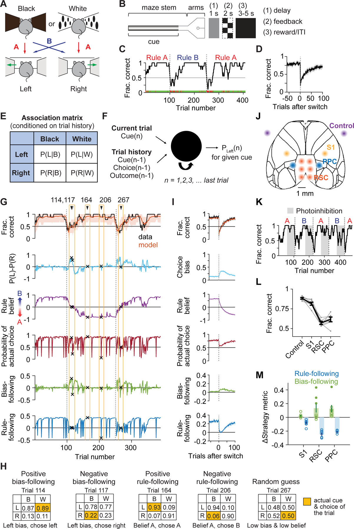
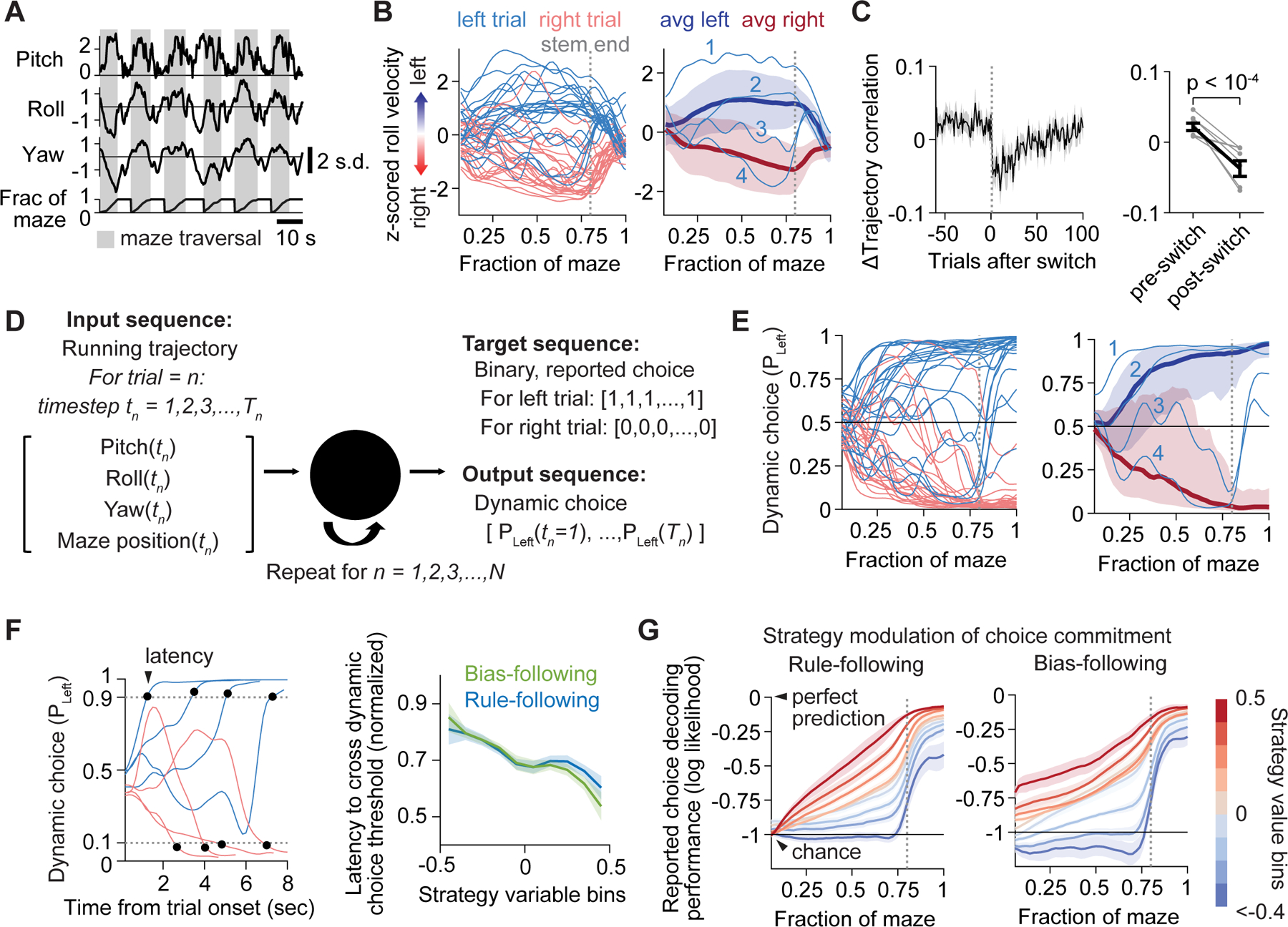
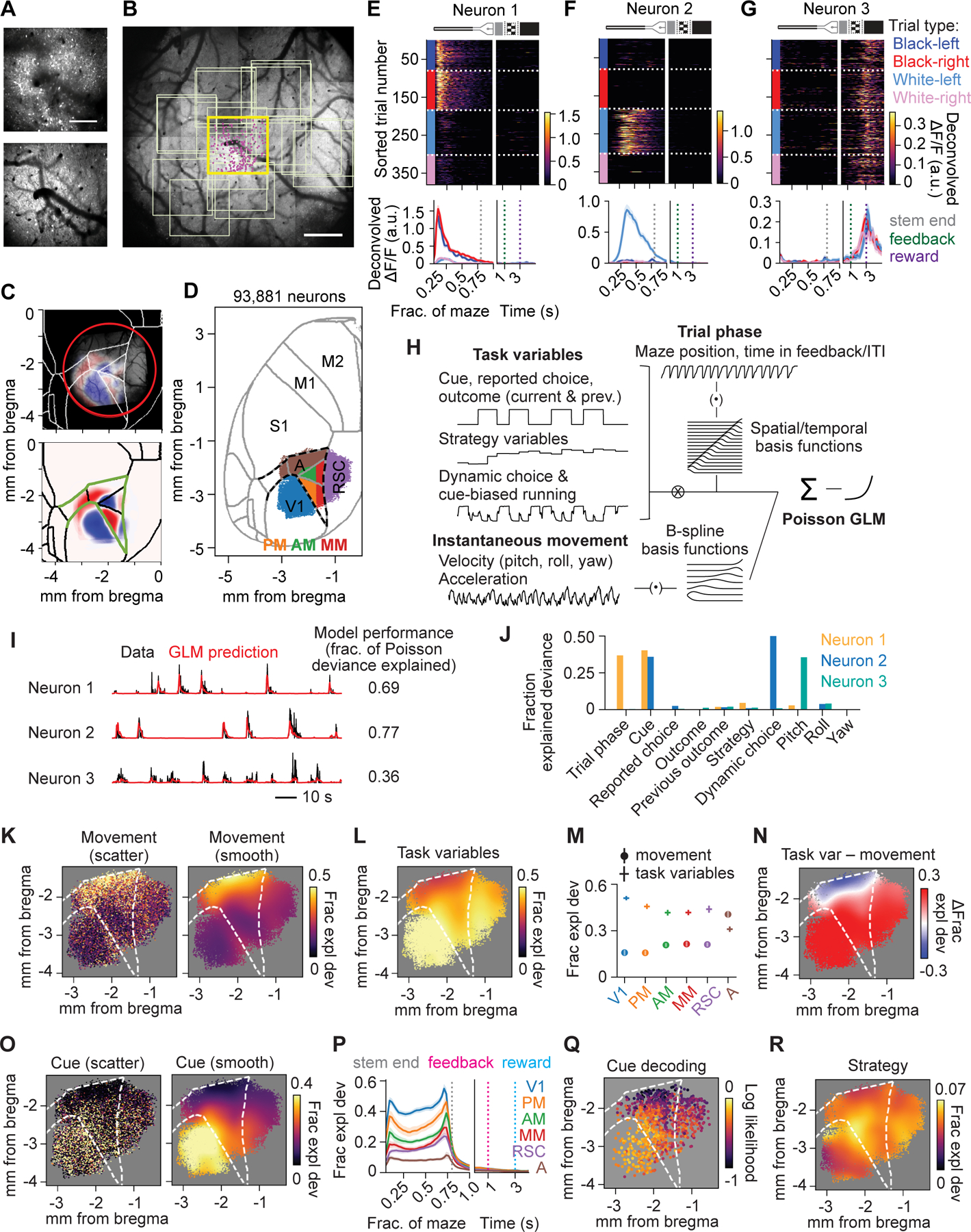
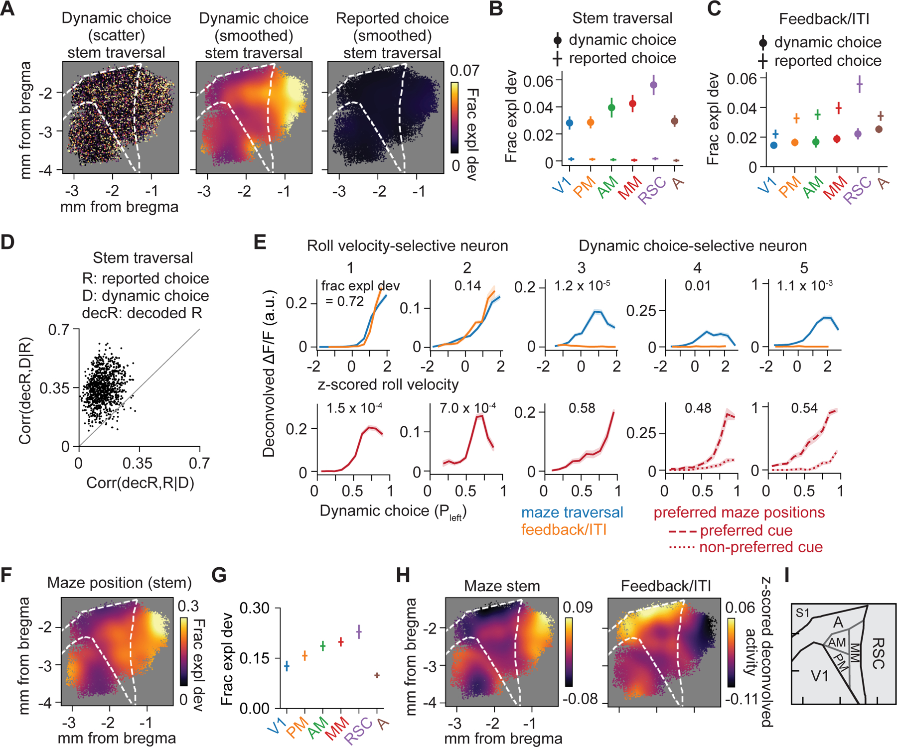
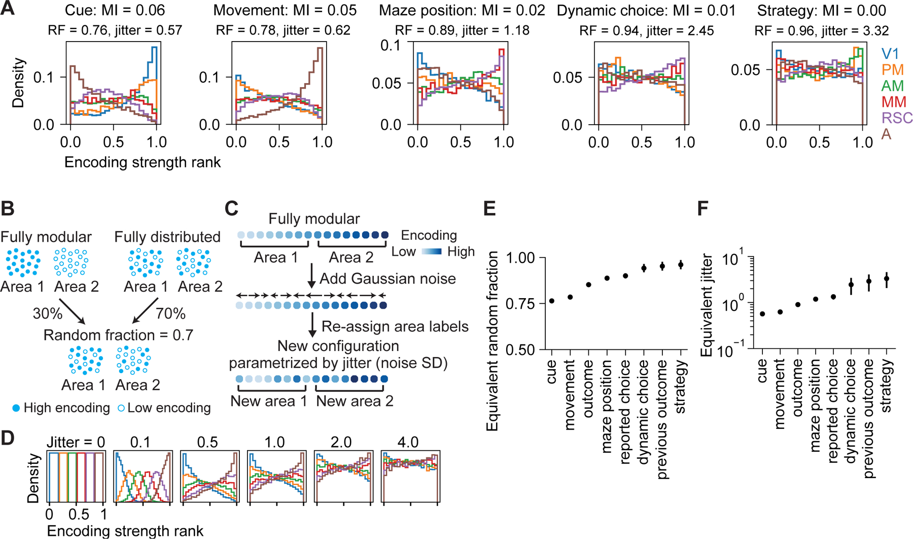
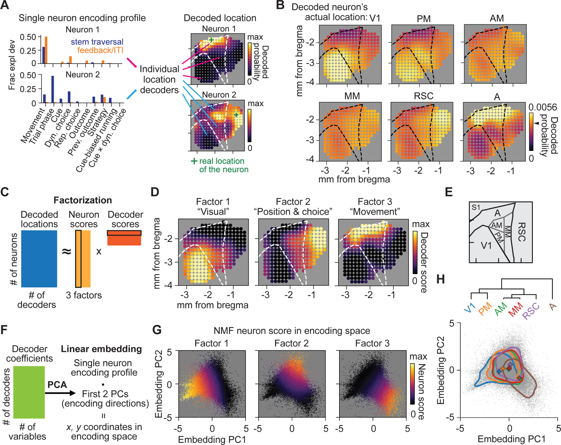
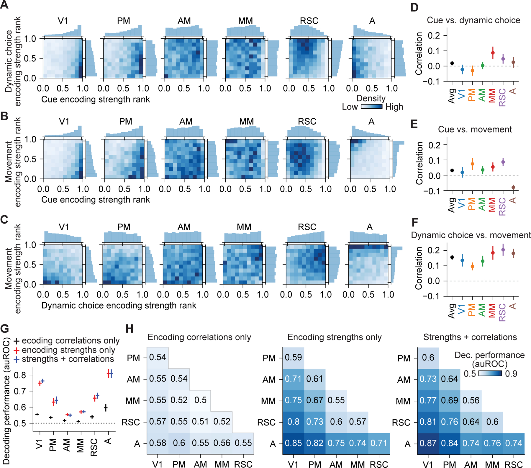
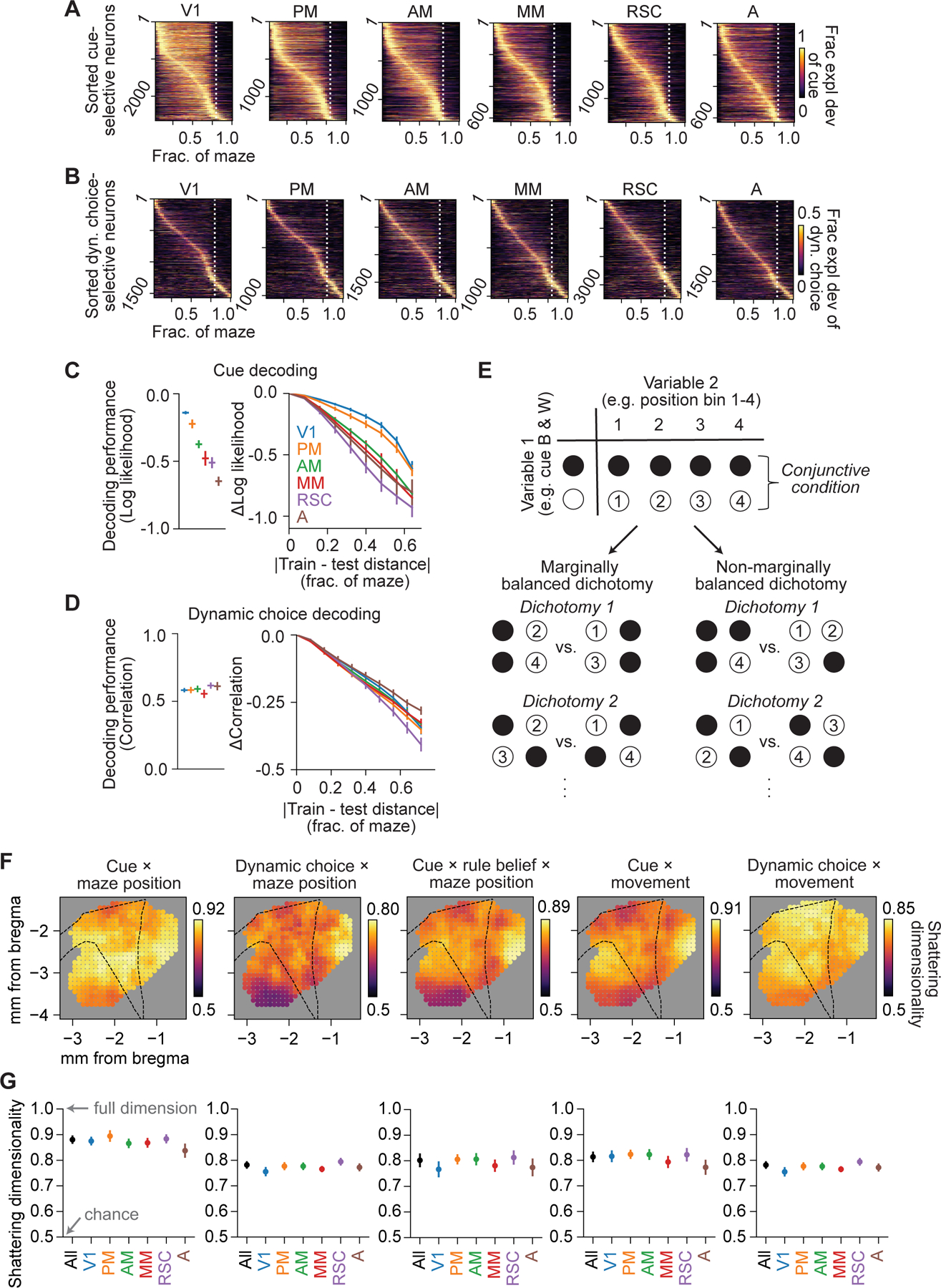
Animals adaptively integrate sensation, planning, and action to navigate toward goal locations in ever-changing environments, but the functional organization of cortex supporting these processes remains unclear. We characterized encoding in approximately 90,000 neurons across the mouse posterior cortex during a virtual navigation task with rule switching. The encoding of task and behavioral variables was highly distributed across cortical areas but differed in magnitude, resulting in three spatial gradients for visual cue, spatial position plus dynamics of choice formation, and locomotion, with peaks respectively in visual, retrosplenial, and parietal cortices. Surprisingly, the conjunctive encoding of these variables in single neurons was similar throughout the posterior cortex, creating high-dimensional representations in all areas instead of revealing computations specialized for each area. We propose that, for guiding navigation decisions, the posterior cortex operates in parallel rather than hierarchically, and collectively generates a state representation of the behavior and environment, with each area specialized in handling distinct information modalities.

Keywords: calcium imaging; conjunctive coding; cortical organization; decision-making; navigation; parietal cortex; population coding; representational geometry; retrosplenial cortex; virtual reality.

Figure 1.. Diverse decision-making strategies during flexible navigation decisions and photoinhibition in posterior cortex

(A) Rewarded cue-choice associations for rules A and B. (B) Maze configuration and structure of trial epochs. At the trial end, after a delay, mice received visual feedback about the correctness before a reward and inter-trial interval. (C) Task performance for an example session. Green ticks, correct trials; red ticks, incorrect trials; black line, smoothed performance (boxcar of 9 trials); gray dashed line, rule switches. (D) Switch-aligned performance. n = 513 switches from 8 mice. (E) Association matrix used to quantify strategy variables: the probability of choosing left or right given a black or white cue for a given trial, conditioned on its trial history. (F) Schematic of LSTM for deriving the association matrix on each trial. (G) Modeled fraction correct and strategy variables for an example session. Orange shading, 90% CI from 1000 simulations of task performance from the model. (H) Association matrices for the 5 example trials in (G). (I) Switch-aligned modeled fraction correct and strategy variables. n = 265 switches. (J) Bilateral inhibition sites in VGAT-ChR2 mice. (K) Task performance of an example session during photoinhibition. (L) Effects of photoinhibition on task performance. Gray lines, individual mice; black line, all mice. Control vs. RSC or PPC: p < 10⁻⁴; control vs. S1: p = 0.0002; S1 vs. RSC or PPC: p < 10⁻⁴; RSC vs. PPC: p = 0.058. n = 164 sessions from 7 mice. (M) Effects of photoinhibition on strategy variables, measured as differences from control. Open circles, average for individual mice. For bias-following, p = 0.025 for S1, p = 0.018 for RSC, p < 10⁻⁴ for PPC; for rule-following, p < 10⁻⁴ for all targets. Filled circles indicate mice with large increase in bias-following (greater than 0.2; 3 mice for RSC and one mouse for PPC). Data and statistics in (D), (I), (L), (M) are presented as hierarchical bootstrap mean ± SEM. See also Figure S1.

Figure 2.. Choice formation estimated from running trajectories

(A) Example normalized treadmill velocities and position in the maze. (B) Roll velocity aligned to maze position. Left: example single trials from one session. Right: four example left trials compared to average left and right trials; mean ± SD. (C) Correlation of running trajectories for choice-matched trials, measured as difference from session average, aligned to the switch (left; n = 265 switches) or averaged for 20 trials before vs. after switches (right; gray lines, individual mice). (D) Schematic of LSTM for decoding reported choice from running trajectories. The output is dynamic choice (P_left). (E) Dynamic choice for same data shown in (B). (F) Left: latency to dynamic choice crossing a threshold (dashed line) for example trials. Right: relationship between latency (normalized by session-averaged trial duration, 8.95 ± 2.04 sec, mean ± SD) and strategy variables. n = 85,463 trials. (G) Time course of choice commitment (LSTM decoding performance for reported choice, calculated as log likelihood with log base 2), binned by values of rule-following (left) and bias-following (right). n = 68,249 trials. Data and statistics in (C), (F), (G) are presented as hierarchical bootstrap mean ± SEM. See also Figure S2.

Figure 3.. Calcium imaging in posterior cortex and encoding of instantaneous movement and task variables

(A) Example mean GCaMP6s image (top) and overlying vasculature pattern near the brain surface (bottom) for an example field of view (FOV). (B) Overview image of the vasculature pattern within the cranial window. Yellow box, location of the FOV in (A); pink dots, locations of neurons recorded in that FOV; light yellow boxes, other FOVs. (C) Top: Registered field sign map overlaid with the vasculature pattern in (B). White lines, area contours from Allen Institute Mouse CCF; red circle, cranial window location. Bottom: Mean field sign map of 8 mice. Green lines: anterior medial border of V1, lateral border of RSC, and posterior border of S1; used as anatomical landmarks in subsequent figures. (D) Parcellation of all recorded neurons into 6 discrete areas, overlaid with area borders from CCF. n = 93,881 neurons from 141 sessions from 8 mice. (E-G) Deconvolved activity of three example RSC neurons. Top: heatmap of single trial activity sorted by trial types. Bottom, trial-type average activity; mean ± SEM. The x-axis is in spatial units during maze traversal and in time units during feedback period/ITI. (H) Schematic of the GLM. (I) Example traces of deconvolved activity and GLM prediction on held-out data for the three neurons shown in (E-G). (J) Encoding profiles (fraction explained deviance for individual variables) of the three neurons in (E-G). (K) Left: encoding magnitude of instantaneous movement for single neurons (individual dots) at their cortical locations. Right: smoothed encoding map (Gaussian filter, SD = 150 μm). n = 42,998 well-fit neurons from 8 mice. (L) Smoothed encoding map for task variables. (M) Average encoding magnitude of instantaneous movement and task variables for 6 areas. Hierarchical bootstrap mean ± SEM. (error bars for movement are contained in the symbols). Area A had higher encoding for movement and lower encoding for task variables than every other area (p < 10⁻³), while V1 had higher encoding for task variables than every other area (p < 10⁻³). (N) Smoothed map showing difference between encoding magnitude of task variables and movement. (O) Left: encoding magnitudes of cue for individual neurons during stem traversal at their cortical locations. Right: smoothed encoding map. (P) Time course of cue encoding for 6 areas for sessions with cue offset at 0.76 of maze length. Hierarchical bootstrap mean ± SEM. (Q) Decoding performance for cue from population activity, quantified as log likelihood with log base 2. Each point represents one population decoder consisting of ~100 nearby neurons, plotted at the mean location of all member neurons. n = 974 decoders. (R) Encoding map of strategy variables, including individual strategy variables and their interactions with task variables. See also Figure S3 and S4.

Figure 4.. Encoding of choice and maze position

(A) Encoding magnitude (left) and smoothed map of dynamic choice (middle) and smoothed map of reported choice (right) during stem traversal. (B) Average encoding magnitude of dynamic choice and reported choice during stem traversal for 6 areas. All 6 areas: dynamic choice vs. reported choice, p < 10⁻³. Dynamic choice: RSC vs. V1, PM or A, p < 10⁻³; RSC vs. AM or MM, p > 0.05. Reported choice: each area vs. zero, p > 0.05. (C) Same as (B), but in feedback period/ITI. All 6 areas: reported choice vs. dynamic choice, p < 10⁻³. Reported choice, RSC vs. each other area, p < 0.05. (D) Partial correlation (Spearman) of decoded reported choice (decR) with dynamic choice (D), conditioned on reported choice (R) (bootstrap mean ± SEM, 0.35 ± 0.02) vs. partial correlation of decR with R, conditioned on D (bootstrap mean ± SEM, 0.14 ± 0.02) during stem traversal. Each point represents one population decoder consisting of ~100 nearby neurons. Mean difference between the two partial correlations is greater than 0 (bootstrap mean difference ± SEM, 0.21 ± 0.02, p < 10⁻³). n = 974 decoders. (E) Tuning curves for roll velocity (top; plotted during maze traversal and feedback period/ITI) and dynamic choice (bottom; plotted at each neuron’s preferred maze position) for two roll velocity-selective neurons (neuron 1 and 2) and three dynamic choice-selective neurons (neuron 3–5). The GLM-derived encoding magnitude (fraction explained deviance) for that variable is indicated on each panel. (F) Smoothed encoding map of maze position during stem traversal. (G) Average encoding magnitude for maze position during stem traversal for 6 areas. RSC vs. V1, PM, or A, p < 10⁻³; RSC vs. AM or MM, p > 0.05. (H) Smoothed maps of average z-scored deconvolved activity during the maze stem (left) and feedback period/ITI (right). (I) Schematic of area parcellation. Data and statistics in (B), (C), (G) are presented as hierarchical bootstrap mean ± SEM. See also Figure S5.

Figure 5.. Distributedness of encoding across posterior cortical areas

(A) Distribution of encoding strength rank of single neurons in 6 areas for various variables. MI, normalized mutual information between encoding strength and area identity; RF: equivalent random fraction; jitter, equivalent jitter; see (B) and (C). (B) Schematic of toy models generated by mixing fully modular and fully distributed configurations with random faction = 0.7. (C) Schematic of toy models generated by perturbing the encoding strength rank of the fully modular configurations by adding Gaussian noise (parametrized by jitter, or Gaussian noise SD) to the rank. (D) Distribution of encoding strength rank for toy models in (C) generated with different jitter values. (E-F) Equivalent random fraction and jitter for various variables. Bootstrap mean ± SEM. See also Figure S6.

Figure 6.. Distinct spatial gradients of encoding in posterior cortex

(A) Examples of decoding cortical locations from GLM-derived encoding profiles of single neurons. (B) For all neurons in one of 6 areas, the average decoded probability distribution of a neuron’s location over posterior cortex. Chance level is 0.0041 (1/number of location decoders; black arrow on the color bar). (C) Schematic of the non-negative factorization (NMF) of the decoded locations of all neurons. (D) NMF decoder scores plotted spatially for each non-negative factor. (E) Schematic of area parcellation. (F) Schematic of embedding of single neuron encoding profiles. (G) All neurons embedded in the encoding space, colored with the NMF neuron scores for each factor. (H) Top: dendrogram showing hierarchical clustering of 6 areas by centroid locations. Bottom: Summary of distribution of neurons in 6 areas in the encoding space. Colored lines, contours at 25% of the peak density; plus signs, centroid locations. See also Figure S6.

Figure 7.. Quantification of encoding correlations showed generic integration

(A) Joint and marginal distributions for encoding strength rank of cue and dynamic choice during stem traversal in 6 areas. (B) Same as (A), but for cue and movement. (C) Same as (A), but for dynamic choice and movement. (D) Pearson correlation between the encoding strength of cue and dynamic choice during stem traversal for neurons in 6 areas. Bootstrap mean ± SEM. Correlations in all areas were not significantly different from one another (p > 0.05). (E) Same as (D), but for cue and movement. A vs. each other area, p < 0.013, whereas correlations in other 5 areas were not significantly different from each other (p > 0.05). (F) Same as (D), but for dynamic choice and movement. Correlations in all areas were not significantly different from one another (p > 0.05). (G) Decoding performance for one-vs.-others decoders that distinguished neurons in each of the 6 areas from neurons in all other areas based on encoding correlations only, encoding strengths only, and both, during stem traversal. Mean ± SEM with leave-one-mouse-out procedure. All decoding was above chance (p < 0.05), except encoding correlations only for PM and AM. Encoding strengths only vs. encoding correlations only: p < 0.05 in all areas except for AM. Encoding strengths only vs. strengths + correlations: p > 0.03 for all areas, not significant after multiple comparison correction. Wilcoxon signed-rank test. (H) Decoding performance for pairwise decoders that distinguished neurons in a pair of areas during stem traversal. See also Figure S7.

Figure 8.. High dimensional representation of conjunctive variables across posterior cortex

(A) Fraction explained deviance of cue for the top 25% cue-selective neurons across all cells, separated in 6 areas and sorted by peak location. (B) Same as (A), except the top 25% of dynamic choice-selective neurons. (C) Left: average decoding performance for cue based on populations of ~100 nearby neurons for 6 areas, quantified as log likelihood with log base 2. Right: change in decoding performance as a function of the distance between maze positions of the data that the decoders were trained on and tested on (restricted to positions where cue was present). n = 698 decoders. (D) Same as (C), but for decoding performance of dynamic choice, quantified as the Spearman correlation between decoded and real values. n = 974 decoders. (E) Schematic for identifying marginally balanced dichotomies over conjunctive conditions formed by a pair of variables. (F) Spatial maps of shattering dimensionality (average decoding accuracy over all marginally balanced dichotomies) during stem traversal. Each dot indicates a population of 1000 nearby neurons centered on that cortical location. (G) Shattering dimensionality based on populations of 1000 neurons subsampled from all neurons and each of the 6 areas. All datapoints were not significantly different from one another (p > 0.01, not significant after multiple comparison correction). Data and statistics in (C), (D), (G) are presented as hierarchical bootstrap mean ± SEM. See also Figure S8.

References

1. Abadi M, Agarwal A, Barham P, Brevdo E, Chen Z, Citro C, Corrado GS, Davis A, Dean J, Devin M, et al. (2016). TensorFlow: Large-Scale Machine Learning on Heterogeneous Distributed Systems. arXiv 10.48550/arXiv.1603.04467. - DOI
1. Akrami A, Kopec CD, Diamond ME, and Brody CD (2018). Posterior parietal cortex represents sensory history and mediates its effects on behaviour. Nature 554, 368–372. - PubMed
1. Alexander AS, and Nitz DA (2015). Retrosplenial cortex maps the conjunction of internal and external spaces. Nat. Neurosci 18, 1143–1151. - PubMed
1. Alexander AS, and Nitz DA (2017). Spatially Periodic Activation Patterns of Retrosplenial Cortex Encode Route Sub-spaces and Distance Traveled. Curr. Biol 27, 1551–1560. - PubMed
1. Allen WE, Kauvar IV, Chen MZ, Richman EB, Yang SJ, Chan K, Gradinaru V, Deverman BE, Luo L, and Deisseroth K (2017). Global Representations of Goal-Directed Behavior in Distinct Cell Types of Mouse Neocortex. Neuron 94, 891–907. - PMC - PubMed
Publication types
LinkOut - more resources