PSegNet: Simultaneous Semantic and Instance Segmentation for Point Clouds of Plants

Abstract

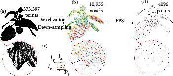
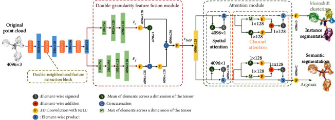
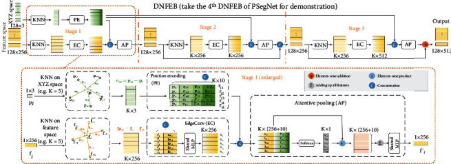
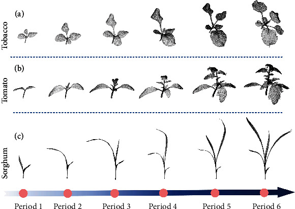
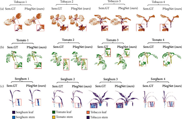
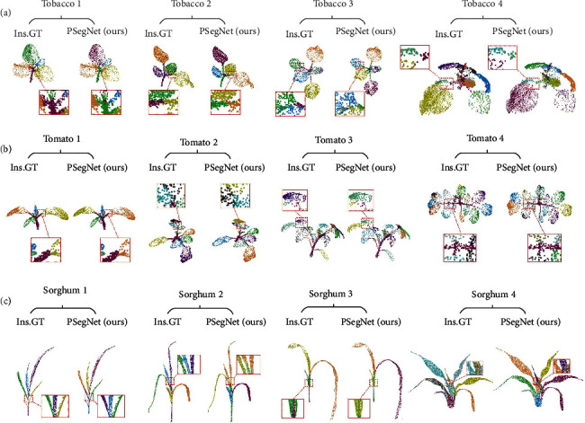
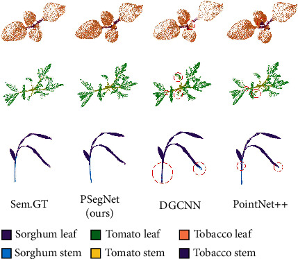
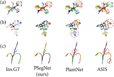
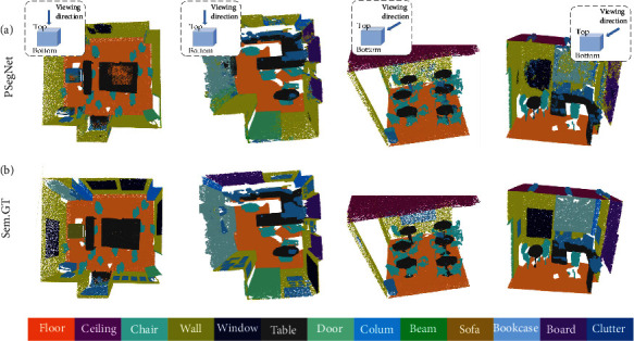
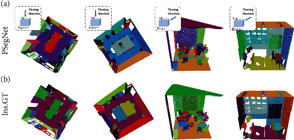
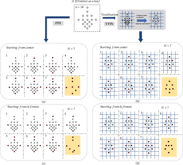
Phenotyping of plant growth improves the understanding of complex genetic traits and eventually expedites the development of modern breeding and intelligent agriculture. In phenotyping, segmentation of 3D point clouds of plant organs such as leaves and stems contributes to automatic growth monitoring and reflects the extent of stress received by the plant. In this work, we first proposed the Voxelized Farthest Point Sampling (VFPS), a novel point cloud downsampling strategy, to prepare our plant dataset for training of deep neural networks. Then, a deep learning network-PSegNet, was specially designed for segmenting point clouds of several species of plants. The effectiveness of PSegNet originates from three new modules including the Double-Neighborhood Feature Extraction Block (DNFEB), the Double-Granularity Feature Fusion Module (DGFFM), and the Attention Module (AM). After training on the plant dataset prepared with VFPS, the network can simultaneously realize the semantic segmentation and the leaf instance segmentation for three plant species. Comparing to several mainstream networks such as PointNet++, ASIS, SGPN, and PlantNet, the PSegNet obtained the best segmentation results quantitatively and qualitatively. In semantic segmentation, PSegNet achieved 95.23%, 93.85%, 94.52%, and 89.90% for the mean Prec, Rec, F1, and IoU, respectively. In instance segmentation, PSegNet achieved 88.13%, 79.28%, 83.35%, and 89.54% for the mPrec, mRec, mCov, and mWCov, respectively.

Figure 1

Schematic diagram of the VFPS strategy. The leftmost point cloud (a) is an original tobacco point cloud that contains a total of 373,397 points. First, we set a number object for downsampled point cloud, e.g., N = 4096. Then, the VBS with parameters l_x = l_y = l_z = 3cm is applied to the original point cloud to form a point cloud (b) containing 10955 voxels. Each voxel is represented by the center of gravity of points in the voxel, and a voxel example is enlarged in (c). At last, FPS is applied on this temporary voxelized point cloud to generate the final result (d) with an exact 4096 points.

Figure 2

The architecture of PSegNet. The network is mainly composed of three parts. The front part has a typical encoder-like structure in deep learning. Four consecutive Double-Neighborhood Feature Extraction Blocks are applied in the front part computation, and the feature space is downsampled before each DNFEB to condense the features, respectively. The middle part is the Double-Granularity Feature Fusion Module, which fuses the outputs of two decoders with different feature granularity to obtain the mixed feature F_DGF. In the third part of PSegNet, the features flow into two directions that, respectively, correspond to two tasks—instance segmentation and semantic segmentation. Spatial attention and channel attention mechanisms are sequentially applied on each feature flow.

Figure 3

Demonstration of DNFEB. The feature dimensions in DNFEB vary with their positions in the PSegNet, and in this figure, we only display feature dimensions of the 4^th DNFEB. A standard DNFEB contains three similar stages. The calculation process of stage 1 is enlarged in the lower part of the figure. On stage 1, for any point i in the feature space, we find its K-nearest neighbors in the initial XYZ space and in the current feature space, respectively. Secondly, position encoding is carried out for K-nearest neighbors in XYZ space to form a low-level feature encoding of the local region. At the same time, EdgeConv is carried out for the K-nearest neighbors in the current feature space to form a high-level feature representation of the local region. Finally, after concatenating the low-level and high-level local features, the new feature vector of the current point i is output after the calculation of the Attentive Pooling operation.

Figure 4

Demonstration of some point clouds from our dataset. (a) Point clouds in 6 consecutive growth periods of the same tobacco plant, respectively; (b) point clouds in 6 consecutive growth periods of the same tomato plant; (c) point clouds in consecutive 6 growth periods of the same sorghum plant.

Figure 5

The changes of losses in the training of PSegNet. From (a–d) are the total loss L, the DHL L_DHL imposed on the midlevel feature layer after DGFMM, the semantic loss L_sem, and the instance loss L_ins . The x-axis of all plots means the number of trained samples, and the y-axis is the loss value. Given 3640 training samples and the training batch size at 8, we have 455 samples to be trained in each epoch. When the training stops at 190 epochs, the x-axis ends at 455∗190 = 86450.

Figure 6

Qualitative demonstration of our PSegNet for semantic segmentation. (a) Semantic segmentation results of four different tobacco individuals, respectively. (b) Semantic segmentation results of four different tomato plants, respectively. (c) Semantic segmentation results of four different sorghum plants, respectively. Each segmented crop point cloud from PSegNet is compared with its corresponding ground truth (Sem.GT). The meanings of different rendered colors are shown at the bottom of the figure. Some of the areas are enlarged to give more details.

Figure 7

The qualitative demonstration of the instance segmentation by PSegNet. (a) Instance segmentation results of four different tobacco individuals, respectively. (b) Instance segmentation results of four different tomato individuals, respectively. (c) Instance segmentation results of four different sorghum individuals, respectively. Each segmented crop point cloud from PSegNet is compared with its corresponding ground truth (Ins.GT). Note that the different rendered colors in this figure are just for better visual separation of different instances, and it has no connection with the instance labels. Therefore, despite successful segmentation, the same leaf instance in the ground truth and the network result may be rendered with two different colors. Some of the areas are enlarged to give more details.

Figure 8

The qualitative semantic segmentation comparison on the three species. DGCNN and PointNet++ are compared with our PSegNet. The parts with segmentation errors are highlighted by red dotted circles, respectively. DGCNN and PointNet++ both have multiple prediction errors around the boundary between two different point classes.

Figure 9

The qualitative instance segmentation comparison on the three species. (a) The tobacco plant and (b) the tomato plant; (c) the sorghum plant. PlantNet and ASIS are compared with our PSegNet. Note that the different rendered colors in this figure are just for better visual effect, and the colors are not associated with the instance labels. The parts with segmentation errors are highlighted by red dotted circles, respectively. PlantNet and ASIS both have multiple prediction errors around the boundaries of leaf instances.

Figure 10

Demonstration of the semantic segmentation results of PSegNet on four different rooms in Area 5 of S3DIS. (a) The semantc prediction results from PSegNet and (b) the semantic ground truth. Different semantic classes are rendered with different colors at the bottom, respectively. The first two rooms are visualized from top, and the third and the fourth rooms are visualized with side views. Each room is composed of several 1 × 1 × he blocks.

Figure 11

Demonstration of the instance segmentation results of PSegNet on four different rooms in Area 5 of S3DIS. (a) The instance prediction results from PSegNet and (b) the instance GT. Different instance classes are rendered with different colors, respectively. Note that the different rendered colors in this figure are just for better visual effect, and the colors are not associated with the instance labels. The first two rooms are visualized from top, and the third and the fourth rooms are visualized with side views. Each room is composed of several 1 × 1 × he blocks.

Figure 12

Comparison of VFPS and FPS on a 2D lattice like a leaf. The original lattice contains 18 points, sparse on the upper part and dense at the lower part. (a) The FPS (N = 7) process starting from the center; (b) the FPS (N = 7) process starting from the leftmost point; (c) VFPS (N = 7) process starting from the center point; (d) VFPS (N = 7) process starting from the leftmost point.

References

1. Li Z., Guo R., Li M., Chen Y., Li G. A review of computer vision technologies for plant phenotyping. Computers and Electronics in Agriculture . 2020;176, article 105672 doi: 10.1016/j.compag.2020.105672. - DOI
1. Trivedi P. Advances in Plant Physiology . IK International Pvt Ltd; 2006.
1. Ogura T., Busch W. Genotypes, networks, phenotypes: moving toward plant systems genetics. Annual Review of Cell and Developmental Biology . 2016;32(1):103–126. doi: 10.1146/annurev-cellbio-111315-124922. - DOI - PubMed
1. Liu H. J., Yan J. Crop genome-wide association study: a harvest of biological relevance. The Plant Journal . 2019;97(1):8–18. doi: 10.1111/tpj.14139. - DOI - PubMed
1. Costa C., Schurr U., Loreto F., Menesatti P., Carpentier S. Plant phenotyping research trends, a science mapping approach. Frontiers in Plant Science . 2019;9:p. 1933. doi: 10.3389/fpls.2018.01933. - DOI - PMC - PubMed
LinkOut - more resources