Empirical transmit field bias correction of T1w/T2w myelin maps

Abstract

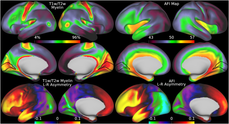
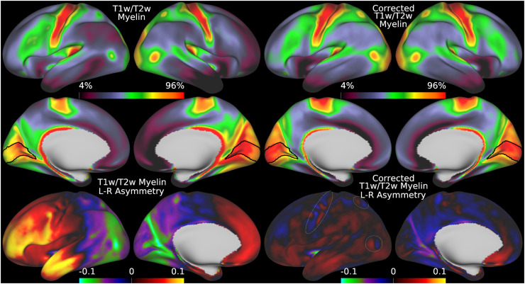
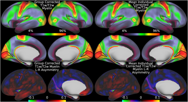
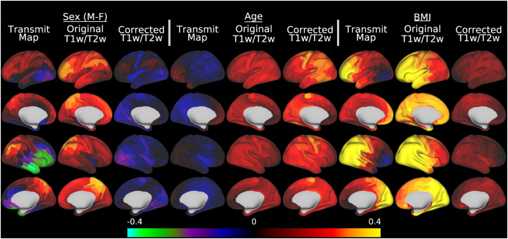
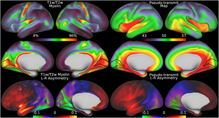
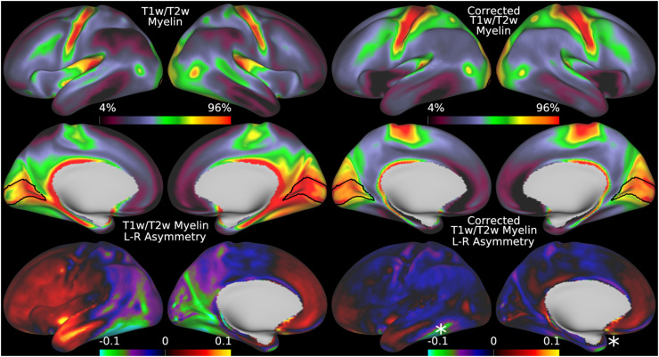
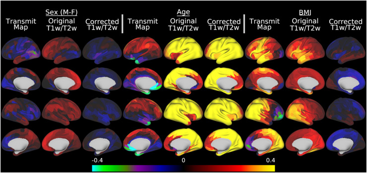
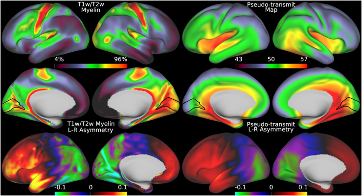
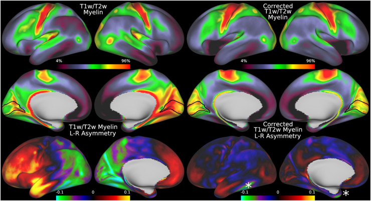
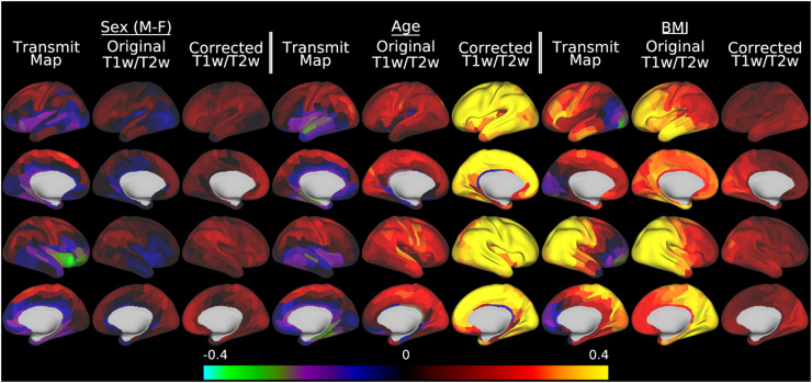
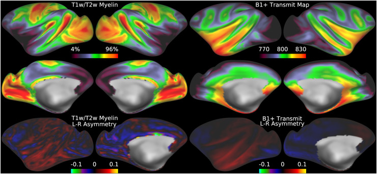
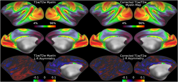
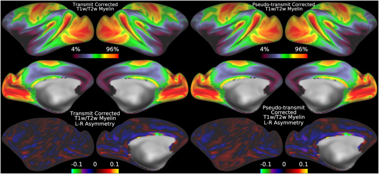
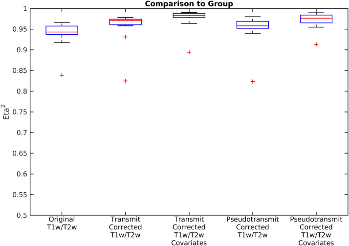
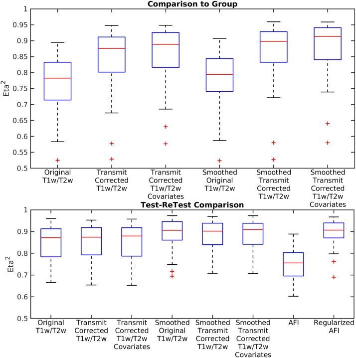
T1-weighted divided by T2-weighted (T1w/T2w) myelin maps were initially developed for neuroanatomical analyses such as identifying cortical areas, but they are increasingly used in statistical comparisons across individuals and groups with other variables of interest. Existing T1w/T2w myelin maps contain radiofrequency transmit field (B1+) biases, which may be correlated with these variables of interest, leading to potentially spurious results. Here we propose two empirical methods for correcting these transmit field biases using either explicit measures of the transmit field or alternatively a 'pseudo-transmit' approach that is highly correlated with the transmit field at 3T. We find that the resulting corrected T1w/T2w myelin maps are both better neuroanatomical measures (e.g., for use in cross-species comparisons), and more appropriate for statistical comparisons of relative T1w/T2w differences across individuals and groups (e.g., sex, age, or body-mass-index) within a consistently acquired study at 3T. We recommend that investigators who use the T1w/T2w approach for mapping cortical myelin use these B1+ transmit field corrected myelin maps going forward.

Fig. 1

illustrates the datasets, specific analyses, and corrected outputs in this study. Bold underlined font indicates the reference T1w/T2w outputs (which are computed only for the surface). Surface data are stored in the CIFTI format (Glasser et al., 2013), which combines both hemispheres into a single file.

Fig. 2

illustrates the overall T1w/T2w transmit field correction pipeline operations and outputs, with inputs and outputs represented by horizontal boxes and processing steps by vertical boxes. Options (depending on specifics of data acquisition) are indicated with different colors (purple for real transmit field, green if Siemens PreScan Normalize (PSN) was used on all images, and blue if motion compensation for the receive field is needed because PSN was not used). Lines that intersect a step (without an arrowhead/passing under the step) skip that particular step. The simplest form of the pipeline (green path) would require that the T1w and T2w images (and GRE/SE images if the pseudo-transmit approach is used) have undergone PSN or the equivalent from another vendor, which permits skipping the Receive Field Correction with Motion Compensation step (blue paths). Bold text indicates the primary outputs of interest for downstream analyses. In all cases, outputs are in CIFTI, NIFTI physical volume, and NIFTI MNI volume spaces.

Fig. 3

illustrates the four optimization approaches used in this study. Each box represents a loop, and anything the box surrounds is inside that loop body. The simplest is the group transmit optimization approach (A), which uses a single loop with the cost function in Eq. 6 and generates species specific reference T1w/T2w myelin maps (the group average B1+ transmit fields are assumed not to require regularization due to cross-participant averaging for removal of artifacts). The reference map is then used in the individual transmit nested optimization algorithm (B) together with the cost function in Eq. 7. The outer loop finds the optimal amount of (spatially constrained) smoothing (for regularization) while compensating for the change in fraction of flip angles above and below the reference flip angle (compensation factor) and the inner loop finds the optimal slope. For the pseudo-transmit approach, the appropriate reference value (the GRE/SE value where the target flip angle is expected to have been achieved by the scanner) must also be found for a given study together with the slope, which is again done at the group level using Eq. 6 with the addition to the cost function of the absolute value of the change in the overall group mean (C). Then the individual pseudo-transmit nested optimization algorithm (D) is used together with the cost function in Eq. 7, with the addition, relative to the individual transmit algorithm (B), of a T2* dropout threshold optimization loop. The reference map from the group transmit algorithm is used in both transmit and pseudo-transmit approaches (because the unregularized pseudo-transmit maps used in (B) have regions with substantial T2* dropout). Appendix A contains a pseudocode representation of the individual pseudo-transmit algorithm.

Fig. 4

illustrates the group average original T1w/T2w volume and the unsmoothed group average AFI map together with unregularized and regularized AFI maps from two exemplar individuals. Panel A shows the group average original T1w/T2w average volume in sagittal (top), coronal (middle) and axial (bottom) slices. Panel B illustrates the group average AFI map, where the original AFI volumes (i.e., TR1 and TR2) are aligned to MNI space nonlinearly and then averaged across participants without smoothing; the AFI flip angle map is then computed from these results at the group level. The arrows mark the anterior and posterior falx and the left tentorium, which all show sharp discontinuities in the AFI map, indicating that the B1+ field is particularly affected by these fibrous dural reflections. Panels C and D illustrate a participant with the worst (worst correlation with the group average map) ringing artifacts before and after regularization. Panel E and F illustrate a participant with the least (best correlation with the group average map) ringing artifacts before and after regularization. Other participants lie between these extremes. Additionally, Panel A shows a subtle correlation with the hemispherically asymmetric pattern in the B1+ map in Panel B within the deep white matter; however, contrast differences between tissues such as CSF/grey matter/white matter are much stronger than those within tissues and also the B1+ effect. This map also illustrates how partial volume effects between CSF/grey matter/white matter tissues overwhelm differences in myelin content within the cortical grey matter in group average T1w/T2w volume maps, making them inappropriate for cortical analyses. Methods sections 2.2 and 2.3 describe the participants and data and preprocessing is described in methods sections 2.6 and 2.7. https://balsa.wustl.edu/PrBrK.

Fig. 5

illustrates the group average T1w/T2w myelin maps (top two rows left), group average AFI maps showing the B1+ field as flip angles (top two rows right, in degrees), left-right asymmetry in T1w/T2w myelin maps (bottom row left), and left-right asymmetry in AFI maps (bottom row right). Area V1 is outlined in black. Methods sections 2.2 and 2.3 describe the participants and data, and preprocessing is described in methods sections 2.6 and 2.7. https://balsa.wustl.edu/7qwq3.

Fig 6

illustrates the group average original T1w/T2w myelin maps (top two rows left), group average corrected T1w/T2w myelin maps (top two rows right), left-right asymmetry in original T1w/T2w myelin maps (bottom row left), and left-right asymmetry in corrected T1w/T2w myelin maps (bottom row right). Area V1 is outlined in black. The faint circles represent the MT+ complex, LIPv, and M1. The L-R cost function (Eq. 6) was used for this correction. Methods sections 2.2 and 2.3 describe the participants and data, and preprocessing is described in methods sections 2.6 and 2.7. https://balsa.wustl.edu/6VjVk.

Fig. 7

illustrates a comparison between the correction applied to the group average and the mean of the individually corrected myelin maps, showing that they are very similar. The data on the left were corrected with the L-R cost function (Eq. 6) and those on the right were corrected with the I-T cost function (Eq. 7). Methods sections 2.2 and 2.3 describe the participants and data and preprocessing is described in methods sections 2.6 and 2.7. https://balsa.wustl.edu/1BgBP.

Fig. 8

illustrates the effect of transmit field correction of individual T1w/T2w myelin maps on a toy statistical model that includes sex, age, and BMI in a multiple linear regression versus the transmit field maps, the original T1w/T2w myelin maps, and the corrected T1w/T2w myelin maps in the HCP-YA data. Within each grouping by variable of interest, standardized beta values enable comparisons across the AFI transmit maps, original T1w/T2w myelin maps, and the B1+ transmit field corrected T1w/T2w myelin maps. For the corrected maps, the covariates of no interest (including the reference voltage, mean transmit field value, 3 transmit field regularization parameters, and corrected CSF regressor, see Methods section 2.10) are included in the model but not illustrated. All of the data were corrected with the I-T cost function (Eq. 7). Methods sections 2.2 and 2.3 describe the participants and data, preprocessing is described in methods sections 2.6 and 2.7, and the analyses are described in methods sections 2.10 and 2.11. https://balsa.wustl.edu/5XqXP.

Fig. 9

shows the original group average T1w/T2w myelin map from the HCD dataset in the top left two rows together with the regularized group average pseudo-transmit field map in the top right two rows. The units of the pseudo-transmit field map are arbitrary, but are scaled similarly to the transmit field map in the prior Fig. 5 to ease comparison. The bottom row shows the corresponding asymmetry maps. Methods sections 2.2 and 2.4 describe the participants and data, and preprocessing is described in methods sections 2.6 and 2.8. https://balsa.wustl.edu/nplpK.

Fig. 10

shows the original group average T1w/T2w myelin map from the HCD dataset in the top left two rows together with the mean corrected individual participant T1w/T2w myelin maps. The bottom row shows the corresponding asymmetry maps. The correction works well for most of the brain, but somewhat less well for areas of high susceptibility where the pseudo-transmit field must be imputed from surrounding valid data (marked with stars). The data on the right were corrected with the I-T cost function (Eq. 7). Methods sections 2.2 and 2.4 describe the participants and data, and preprocessing is described in methods sections 2.6 and 2.8. https://balsa.wustl.edu/g767V.

Fig. 11

illustrates the effect of pseudo-transmit field correction of individual T1w/T2w myelin maps on a toy statistical model that includes sex, age, and BMI in a multiple linear regression versus the pseudo-transmit field maps, the original T1w/T2w myelin maps, and the corrected T1w/T2w myelin maps in the HCD data. Within each grouping by variable of interest, standardized beta values enable comparisons across the pseudo-transmit maps, original T1w/T2w myelin maps, and the pseudo-transmit field corrected T1w/T2w myelin maps. For the corrected maps, the covariates of no interest (including the reference voltage, mean transmit field value, 4 transmit field regularization parameters, and corrected CSF regressor, see Methods section 2.10) are included in the model but not illustrated. All of the data were corrected with the I-T cost function (Eq. 7). Methods sections 2.2 and 2.4 describe the participants and data, preprocessing is described in methods sections 2.6 and 2.8, and the analyses are described in methods sections 2.10 and 2.11. https://balsa.wustl.edu/Mxnx8.

Fig. 12

shows the original group average T1w/T2w myelin map from the HCA dataset in the top left two rows together with the regularized group average pseudo-transmit field map in the top right two rows. The units of the pseudo-transmit field map are arbitrary, but are scaled similarly to the transmit field map in the prior Fig. 5 to ease comparison. The bottom row shows the corresponding asymmetry maps. Methods sections 2.2 and 2.4 describe the participants and data, and preprocessing is described in methods sections 2.6 and 2.8. https://balsa.wustl.edu/B494V.

Fig. 13

shows the original group average T1w/T2w myelin map from the HCA dataset in the top left two rows together with the mean pseudo-transmit corrected individual participant T1w/T2w myelin maps. The bottom row shows the corresponding asymmetry maps, with stars marking areas of high susceptibility where the pseudo-transmit field must be imputed from surrounding valid data. The data on the right were corrected with the I-T cost function (Eq. 7). Methods sections 2.2 and 2.4 describe the participants and data, and preprocessing is described in methods sections 2.6 and 2.8. https://balsa.wustl.edu/lLMLp.

Fig. 14

illustrates the effect of pseudo-transmit field correction of individual T1w/T2w myelin maps on a toy statistical model that includes sex, age, and BMI in a multiple linear regression versus the pseudo-transmit field maps, the original T1w/T2w myelin maps, and the corrected T1w/T2w myelin maps in the HCA data. Within each grouping by variable of interest, standardized beta values enable comparisons across the pseudo-transmit transmit maps, original T1w/T2w myelin maps, and the pseudo-transmit field corrected T1w/T2w myelin maps. For the corrected maps, the covariates of no interest (including the reference voltage, mean transmit field value, 4 transmit field regularization parameters, and corrected CSF regressor, see Methods section 2.10) are included in the model but not illustrated. All of the data were corrected with the I-T cost function (Eq. 7). Methods sections 2.2 and 2.4 describe the participants and data, preprocessing is described in methods sections 2.6 and 2.8, and the analyses are described in methods sections 2.10 and 2.11. https://balsa.wustl.edu/qNwNZ.

Fig. 15

illustrates the group average T1w/T2w myelin maps (top two rows left), group average B1+ transmit field maps (top two rows right), left-right asymmetry in T1w/T2w myelin maps (bottom row left), and left-right asymmetry in group average B1+ transmit field maps (bottom row right) of the NHP_NNP data. The units of the B1+ transmit field map are flip angle * 10, as generated by the scanner with a reference flip angle of 80 degrees instead of 50 degrees as in humans. Methods sections 2.2 and 2.5 describe the participants and data, and preprocessing is described in methods sections 2.6 and 2.9. https://balsa.wustl.edu/jjnjZ.

Fig. 16

illustrates the group average original T1w/T2w myelin maps (top two rows left), group average B1+ transmit field corrected T1w/T2w myelin maps (top two rows right), left-right asymmetry in original T1w/T2w myelin maps (bottom row left), and left-right asymmetry in corrected T1w/T2w myelin maps (bottom row right) of the NHP_NNP data. The L-R cost function (Eq. 6) was used for this correction. Methods sections 2.2 and 2.5 describe the participants and data, and preprocessing is described in methods sections 2.6 and 2.9. https://balsa.wustl.edu/wNzNZ.

Fig. 17

illustrates mean individual transmit field (top left two rows) and pseudo-transmit field (top right two rows) corrected T1w/T2w myelin maps of the NHP_NNP data. The corresponding asymmetry maps are shown in the bottom left and right row respectively. All of the data were corrected with the I-T cost function (Eq. 7). Methods sections 2.2 and 2.5 describe the participants and data, and preprocessing is described in methods sections 2.6 and 2.9https://balsa.wustl.edu/4mlml.

Fig. 18

shows boxplots of the eta² between the group average corrected reference T1w/T2w myelin map and the individual T1w/T2w myelin maps for the n=16 macaque datasets. This is shown for the original T1w/T2w myelin values, the transmit field corrected T1w/T2w myelin values without and with covariate regression, and the pseudo-transmit field corrected T1w/T2w myelin values without and with covariate regression. The red line is the median, the edges of the box are the 25th and 75th percentiles (the interquartile range, IQR), the whiskers extend from the end of the IQR to the furthest observation within 1.5 * IQR, and the outliers (+’s) are the data points beyond those limits. The range of eta² is 0-1, with identical inputs yielding 1; inputs that are strictly the negative of each other yielding 0; and values in between represent varying degrees of 'similarity' (with 0.5 meaning no relationship). All of the data were corrected with the I-T cost function (Eq. 7). Methods sections 2.2 and 2.5 describe the participants and data, and preprocessing is described in methods sections 2.6, 2.9, 2.10, and 2.12.

Fig. 19

shows box plots across HCP-YA test-retest participants (n=41). Along the top row the eta² between each scan and the reference group average corrected myelin map is illustrated for both the ‘Test’ and ‘ReTest’ visits of the Test-ReTest participants. This is shown for the original T1w/T2w myelin values, the transmit field corrected T1w/T2w myelin values without and with covariate regression, and the transmit field corrected T1w/T2w myelin values without and with covariate regression with smoothing. Along the bottom row, the eta² between the Test and ReTest data is shown for each measure including unregularized and regularized AFI. Smoothing is 4mm FWHM on the surface, which improves test-retest reproducibility somewhat due to reduction in variability from random noise and small surface reconstruction differences. All of the data were corrected with the I-T cost function (Eq. 7). Methods sections 2.2 and 2.3 describe the participants and data, and preprocessing is described in methods sections 2.6, 2.7, 2.10, and 2.12.

Fig. 20

illustrates the group average T1w/T2w map after B1+ correction from the HCP-YA data. The L-R cost function (Eq. 6) was used for this correction. Methods sections 2.2 and 2.3 describe the participants and data, and preprocessing is described in methods sections 2.6., 2.7, and 2.13. https://balsa.wustl.edu/mDBD3. Corresponding uncorrected data is available in the BALSA scene.

References

1. Arshad M., Stanley J.A., Raz N. Test–retest reliability and concurrent validity of in vivo myelin content indices: Myelin water fraction and calibrated T1w/T2w image ratio. Hum. Brain Mapp. 2017;38(4):1780–1790. - PMC - PubMed
1. Autio J.A., Glasser M.F., Ose T., Donahue C.J., Bastiani M., Ohno M., Kawabata Y., Urushibata Y., Murata K., Nishigori K., Yamaguchi M. Towards HCP-Style macaque connectomes: 24-Channel 3T multi-array coil, MRI sequences and preprocessing. Neuroimage. 2020;215 - PMC - PubMed
1. Baum G., Flournoy J., Glasser M.F, Harms M., Mair P., Sanders A., Barch D., Buckner R., Bookheimer S., Dapretto M., Smith S., Thomas K., Yacoub E., Van Essen D., Somerville L. Graded variation in cortical T1w/T2w myelination during adolescence. Journal of Neuroscience. 2022 - PMC - PubMed
1. Bock N.A., Hashim E., Janik R., Konyer N.B., Weiss M., Stanisz G.J., Turner R., Geyer S. Optimizing T1-weighted imaging of cortical myelin content at 3.0T. Neuroimage. 2013;65:1–12. - PubMed
1. Bonny J.M., Foucat L., Laurent W., Renou J.P. Optimization of signal intensity andt1-dependent contrast with nonstandard flip angles in spin-echo and inversion-recovery mr imaging. J. Magn. Reson. 1998;130(1):51–57. - PubMed
Publication types