NNMT: Mean-Field Based Analysis Tools for Neuronal Network Models

Abstract

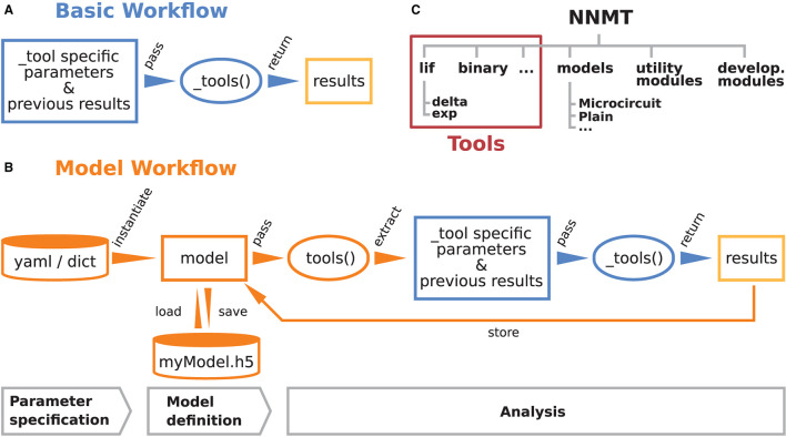
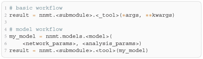
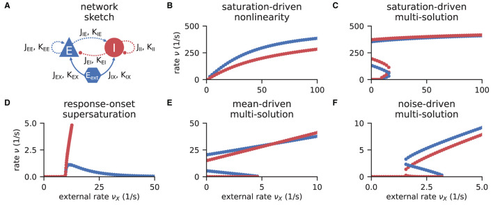
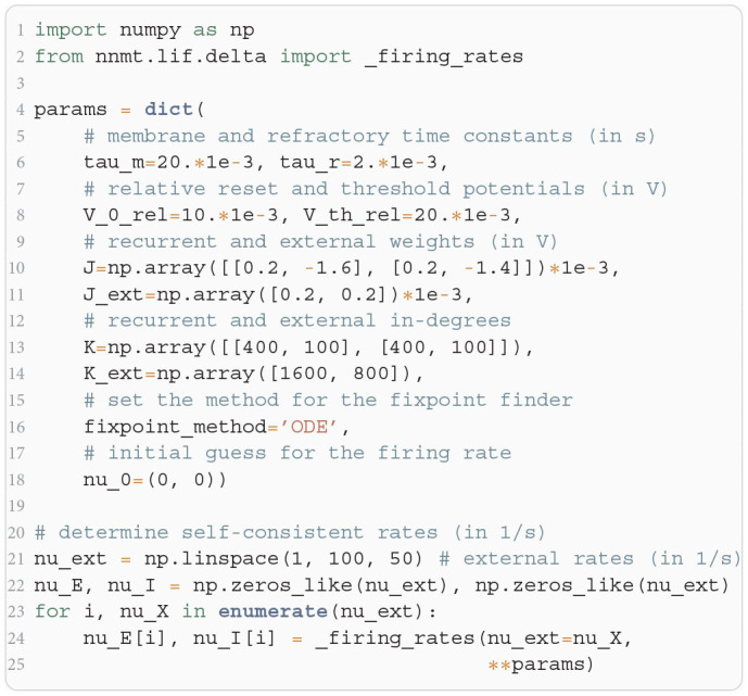
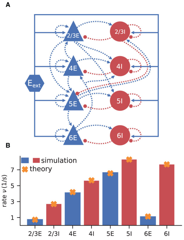
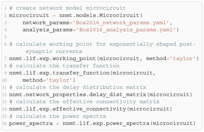
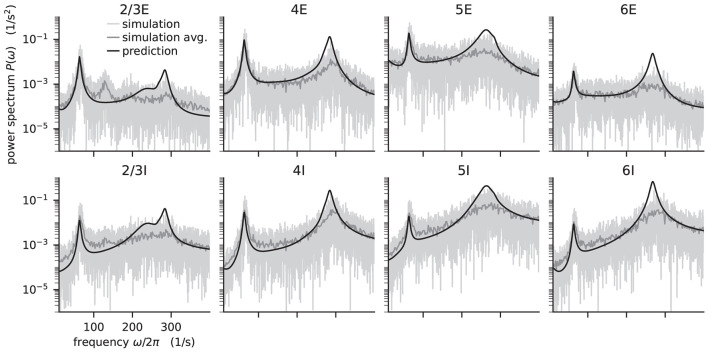
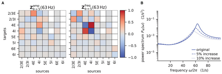
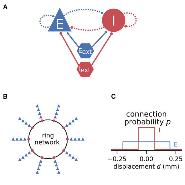
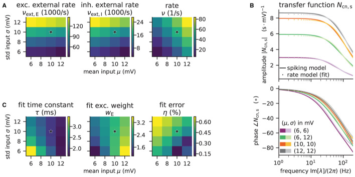
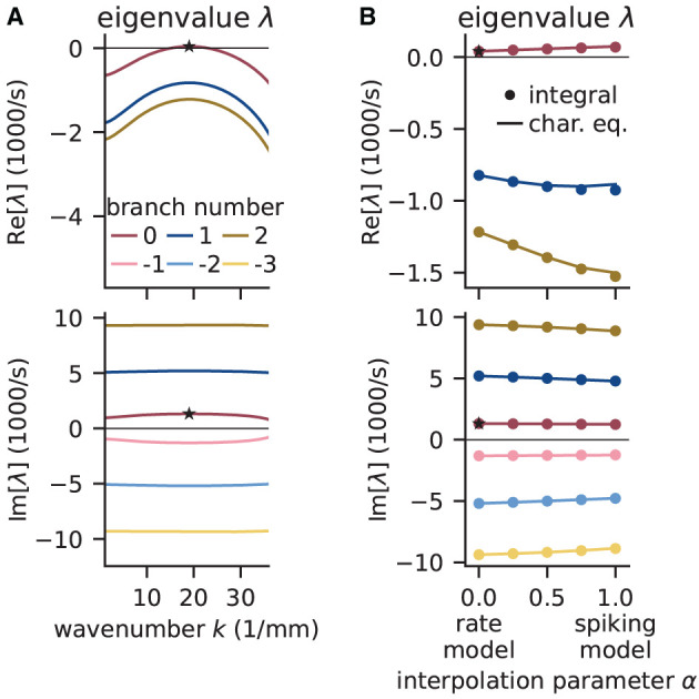
Mean-field theory of neuronal networks has led to numerous advances in our analytical and intuitive understanding of their dynamics during the past decades. In order to make mean-field based analysis tools more accessible, we implemented an extensible, easy-to-use open-source Python toolbox that collects a variety of mean-field methods for the leaky integrate-and-fire neuron model. The Neuronal Network Mean-field Toolbox (NNMT) in its current state allows for estimating properties of large neuronal networks, such as firing rates, power spectra, and dynamical stability in mean-field and linear response approximation, without running simulations. In this article, we describe how the toolbox is implemented, show how it is used to reproduce results of previous studies, and discuss different use-cases, such as parameter space explorations, or mapping different network models. Although the initial version of the toolbox focuses on methods for leaky integrate-and-fire neurons, its structure is designed to be open and extensible. It aims to provide a platform for collecting analytical methods for neuronal network model analysis, such that the neuroscientific community can take maximal advantage of them.

Keywords: (hybrid) modeling; (spiking) neuronal network; computational neuroscience; integrate-and-fire neuron; mean-field theory; open-source software; parameter space exploration; python.

Figure 1

Structure and workflows of the Neuronal Network Mean-field Toolbox (NNMT). (A) Basic workflow: individual mean-field based analysis methods are implemented as functions, called _tools(), that can be used directly by explicitly passing the required arguments. (B) Model workflow: to facilitate the handling of parameters and results, they can be stored in a model class instance, which can be passed to a tool(), which wraps the basic workflow of the respective _tool(). (C) Structure of the Python package. In addition to the tool collection (red frame), containing the tools() and the _tools(), and pre-defined model classes, the package provides utility functions for handling parameter files and unit conversions, as well as software aiding the implementation of new methods.

Listing 1

The two modes of using NNMT: In the basic workflow (top), quantities are calculated by passing all required arguments directly to the underscored tool functions available in the submodules of NNMT. In the model workflow (bottom), a model class is instantiated with parameter sets and the model instance is passed to the non-underscored tool functions which automatically extract the relevant parameters.

Figure 2

Response nonlinearities in EI-networks. (A) Network diagram with nodes and edges according to the graphical notation proposed by Senk et al. (in press). (B–F) Firing rate of excitatory (blue) and inhibitory (red) population for varying external input rate ν_X. Specific choices for synaptic weights (J, J_ext) and in-degrees (K, K_ext) lead to five types of nonlinearities: (B) saturation-driven nonlinearity, (C) saturation-driven multi-solution, (D) response-onset supersaturation, (E) mean-driven multi-solution, and (F) noise-driven multi-solution. See Figure 8 in Sanzeni et al. (2020) for parameters.

Listing 2

Example script to produce the data shown in Figure 2B using the ODE method (initial value ν_a,0 = 0 for population a ∈ {E, I}).

Figure 3

Cortical microcircuit model by Potjans and Diesmann (2014). (A) Network diagram (only the strongest connections are shown as in Figure 1 of the original publication). Same notation as in Figure 2A. (B) Simulation and mean-field estimate for average population firing rates using the parameters from Bos et al. (2016).

Listing 3

Some microcircuit network parameters defined in a yaml file. A dictionary-like structure with the keys val (value) and unit is used to define the membrane time constant, which is the same across all populations. The numbers of neurons in each population are defined as a list. Only the numbers for the first three populations are displayed.

Figure 4

Colored-noise transfer function N_cn of LIF model in different regimes. (A) Absolute value and (B) phase of the “shift” version of the transfer function as a function of the log-scaled frequency. Neuron parameters are set to V_th = 20 mV, V₀ = 15 mv, τ_m = 20 ms, and τ_s = 0.5 ms. For given noise intensities of input current, σ = 4 mV (solid line) and σ = 1.5 mV (dashed line), the mean input μ is chosen such that firing rates ν = 10 Hz (black) and ν = 30 Hz (gray) are obtained.

Listing 4

Example script for computing a transfer function shown in Figure 4 using the method of shifted integration boundaries.

Listing 5

Example script to produce the theoretical prediction (black lines) shown in Figure 5B.

Figure 5

Power spectra of the population spiking activity in the adapted cortical microcircuit from Bos et al. (2016). The spiking activity of each population in a 10 s simulation of the model is binned with 1 ms resolution and the power spectrum of the resulting histogram is calculated by a fast Fourier transform (FFT; light gray curves). In addition, the simulation is split into 500 ms windows, the power spectrum calculated for each window and averaged across windows (gray curves). Black curves correspond to analytical prediction obtained with NNMT as described in Listing 5. The panels show the spectra for the excitatory (top) and inhibitory (bottom) populations within each layer of the microcircuit.

Figure 6

Sensitivity measure at low-γ frequency and corresponding power spectrum of microcircuit with adjusted connectivity. (A) Sensitivity measure of one eigenmode of the effective connectivity relevant for low-γ oscillations. The sensitivity measure for this mode is evaluated at the frequency where the corresponding eigenvalue is closest to the point of instability 1 + 0i in complex plane. $Z_b^{\mathrm{\text{amp}}}(\omega )$ (left subpanel) visualizes the influence of a perturbation of a connection on the peak amplitude of the power spectrum. $Z_b^{\mathrm{\text{freq}}}(\omega )$ (right subpanel) shows the impact on the peak frequency. Non-existent connections are masked white. (B) Mean-field prediction of power spectrum of population 4I with original connectivity parameters (solid line), 5% increase (dashed line) and 10% increase (dotted line) in connections K_{4I → 4I}. The increase in inhibitory input to population 4I was counteracted by an increase of the excitatory external input K_{ext → 4I} to maintain the working point.

Figure 7

Illustrations of spiking network model by Senk et al. (2020). (A) Excitatory and inhibitory neuronal populations randomly connected with fixed in-degree and multapses allowed (autapses prohibited). External excitatory and inhibitory Poisson drive to all neurons. Same notation as in Figure 2A. (B) One inhibitory and four excitatory neurons per grid position on a one-dimensional domain with periodic boundary conditions (ring network). (C) Normalized, boxcar-shaped connection probability with wider excitation than inhibition; the grid spacing is here 10⁻³ mm. For model details and parameters, see Tables II–IV of Senk et al. (2020); the specific values given in the caption of their Figure 6 are used throughout here.

Figure 8

Network parameters and mean-field results from scanning through different working points. Working point (μ, σ) combines mean input μ and noise intensity of input σ. (A) External excitatory ν_ext,E and inhibitory ν_ext,I Poisson rates required to set (μ, σ) and resulting firing rates ν. (B) Transfer function N_cn,s of spiking model and fitted rate-model approximation with low-pass filter for selected (μ, σ) (top: amplitude, bottom: phase). (C) Fit results (time constants τ and excitatory weights w_E) and fit errors η. The inhibitory weights are w_I = −gw_E with g = 5. Star marker in panels (A) and (C) denotes target working point (10, 10) mV. Similar displays as in Senk et al. (, Figure 5).

Figure 9

Linear stability analysis of spatially structured network model. (A) Analytically exact solution for real (top) and imaginary (bottom) part of eigenvalue λ vs. wavenumber k using rate model derived by fit of spiking model at working point (μ, σ) = (10, 10) mV. Color-coded branches of Lambert W_B function; maximum real eigenvalue (star marker) on principal branch (B = 0). (B) Linear interpolation between rate (α = 0) and spiking model (α = 1) by numerical integration of Senk et al. (, Equation 30) (solid line) and by numerically solving the characteristic equation in Senk et al. (, Equation 29) (circular markers). Star markers at same data points as in (A). Similar displays as in Senk et al. (, Figure 6).

References

1. Abramowitz M., Stegun I. A. (1974). Handbook of Mathematical Functions: With Formulas, Graphs, and Mathematical Tables (New York: Dover Publications; ).
1. Ahmadian Y., Miller K. D. (2021). What is the dynamical regime of cerebral cortex? Neuron 109, 3373–3391. 10.1016/j.neuron.2021.07.031 - DOI - PMC - PubMed
1. Amari S.-I. (1975). Homogeneous nets of neuron-like elements. Biol. Cybern. 17, 211–220. 10.1007/BF00339367 - DOI - PubMed
1. Amari S.-I. (1977). Dynamics of pattern formation in lateral-inhibition type neural fields. Biol. Cybern. 27, 77–87. 10.1007/bf00337259 - DOI - PubMed
1. Amit D. J., Brunel N. (1997a). Dynamics of a recurrent network of spiking neurons before and following learning. Netw. Comp. Neural Sys. 8, 373–404. 10.1088/0954-898x_8_4_003 - DOI - PubMed