Isotachophoresis: Theory and Microfluidic Applications

Abstract

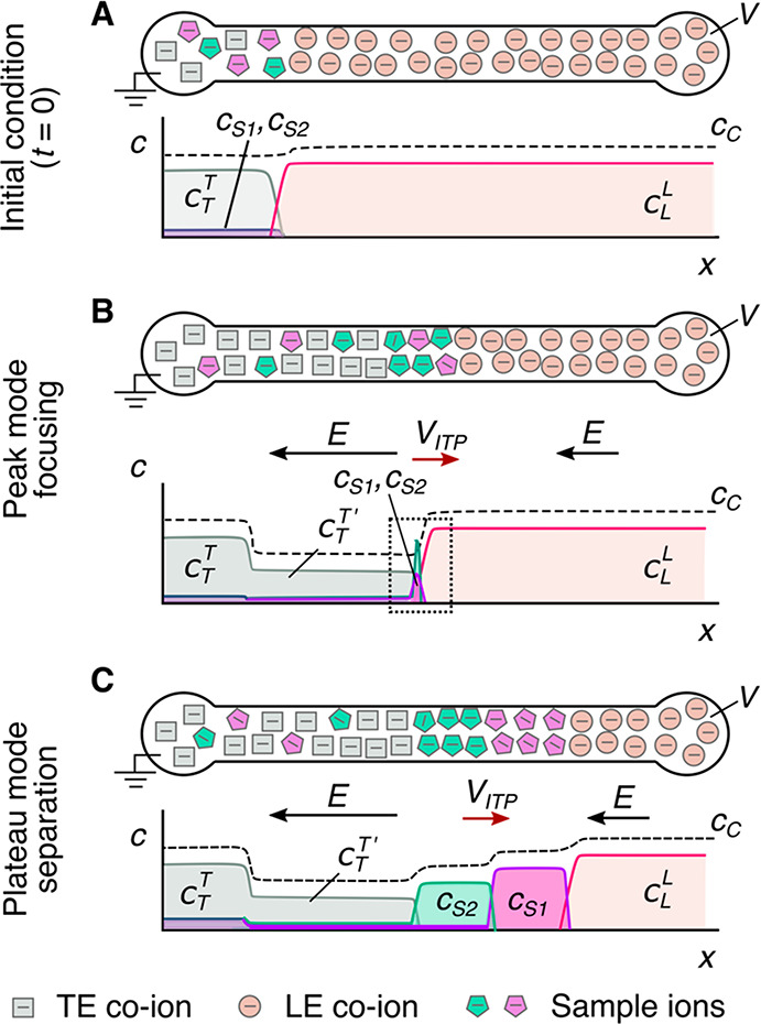
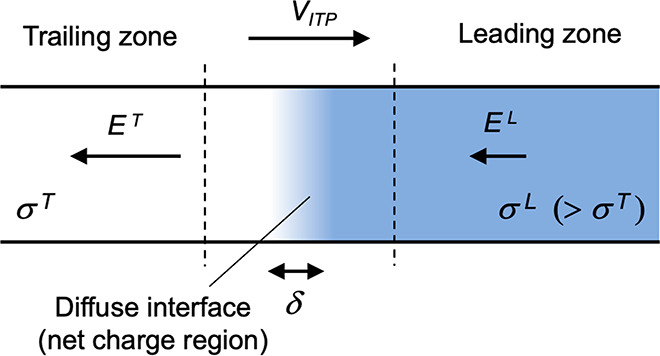
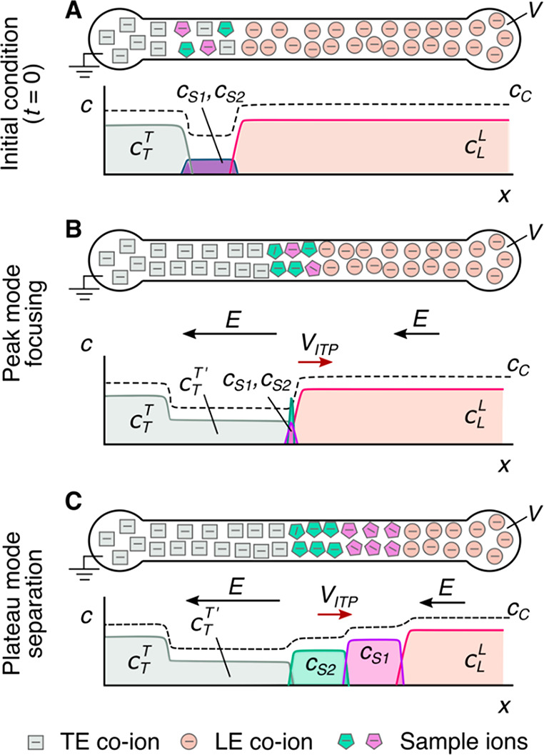
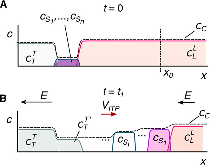
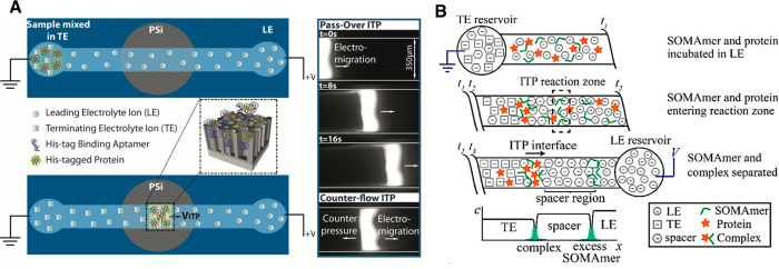
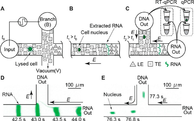
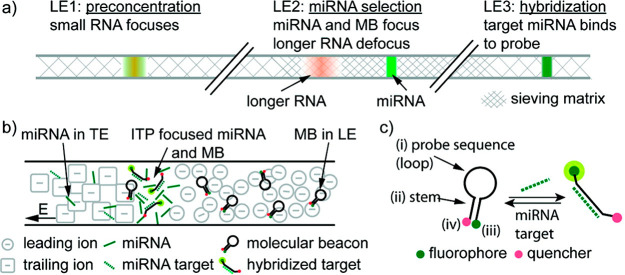
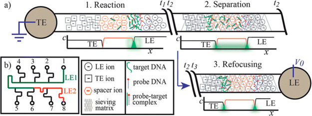
Isotachophoresis (ITP) is a versatile electrophoretic technique that can be used for sample preconcentration, separation, purification, and mixing, and to control and accelerate chemical reactions. Although the basic technique is nearly a century old and widely used, there is a persistent need for an easily approachable, succinct, and rigorous review of ITP theory and analysis. This is important because the interest and adoption of the technique has grown over the last two decades, especially with its implementation in microfluidics and integration with on-chip chemical and biochemical assays. We here provide a review of ITP theory starting from physicochemical first-principles, including conservation of species, conservation of current, approximation of charge neutrality, pH equilibrium of weak electrolytes, and so-called regulating functions that govern transport dynamics, with a strong emphasis on steady and unsteady transport. We combine these generally applicable (to all types of ITP) theoretical discussions with applications of ITP in the field of microfluidic systems, particularly on-chip biochemical analyses. Our discussion includes principles that govern the ITP focusing of weak and strong electrolytes; ITP dynamics in peak and plateau modes; a review of simulation tools, experimental tools, and detection methods; applications of ITP for on-chip separations and trace analyte manipulation; and design considerations and challenges for microfluidic ITP systems. We conclude with remarks on possible future research directions. The intent of this review is to help make ITP analysis and design principles more accessible to the scientific and engineering communities and to provide a rigorous basis for the increased adoption of ITP in microfluidics.

Figure 1

Schematics for the qualitative understanding of microfluidic ITP. (A) Initial conditions at t = 0, common to both peak- and plateau-mode ITP. (B) Peak-mode ITP focusing, which corresponds to either trace analyte focusing or the early stages of any ITP focusing (cf. sections 2.7 and 5). (C) Plateau-mode ITP for the case where the analytes are present in high concentrations and the experiment is run for a sufficiently long duration (cf. sections 2.7 and 6). Each subfigure shows the locations of ions within the channel (top) and the concentration profiles of the electrolytes (bottom) in anionic ITP. For illustration, only two sample species S₁ and S₂ are considered. Peak-mode sample concentration fields are exaggerated for depiction, while sample-mode concentration fields are drawn to relative scale. The loading configuration depicted in panel A, and the schematics in panels B and C correspond to a semi-infinite sample loading configuration (cf. section 2.7).

Figure 2

Simple one-dimensional treatment of an ITP interface. The diffuse interface between the two region has a length scale δ. The regions away from the interface have locally uniform conductivities σ^L and σ^T. Current conservation requires a sharp gradient in the electric field and therefore a local net charge.

Figure 3

Schematic of the finite sample injection configuration for microfluidic ITP. (A) Initial placement of the LE, the TE, and the sample, common to both peak- and plateau-mode ITP. (B and C) Peak- and plateau-mode ITP focusing, respectively. Each subfigure shows the locations of ions within the channel (top) and the concentration profiles of the electrolytes (bottom) in anionic ITP. For finite injection, when the experiment is sufficiently long, all sample ions focus in ITP, leading to steady-state concentration fields of focused ions. This is unlike the case of semi-infinite injection (Figure 1), which is associated with continuous sample focusing in ITP (i.e., the focused sample amount increases with time).

Figure 4

Concentration profiles for strong electrolytes in plateau-mode ITP. (A) Finite injection sample loading configuration. The sample contains a mixture of ions S₁, ..., S_n, which focus in ITP. (B) Sample ions are focused and stack in the descending order of (magnitude of) mobility values between the LE and the TE. The vertical dashed line in panel A indicates an example location along the channel where we chose to illustrate the application of the Kohlrausch regulating function, as shown in section 3.5. The S₁ ion and counterion at x = x₀ must meet the KRF set by the LE zone that originally occupied this region.

Figure 5

Simulated cationic ITP run for a LE mixture consisting of 10 mM potassium ions and 5 mM sulfate ions and for a TE mixture consisting of 10 mM sodium ions and 5 mM sulfate ions. (A and C) Concentration fields at t = 0 and t = 1.1 s, respectively. (B and D) Value of the Kohlrausch regulating function (KRF) versus the channel location x at t = 0 and t = 1.1 s, respectively. Simulations were performed using Simul software with the following parameters: a capillary length of 3 mm, a driving voltage of 50 V, and an x-coordinate mesh consisting of 1000 nodes. The figure was reproduced with permission from ref (136). Copyright 2007 John Wiley and Sons.

Figure 6

Schematic of plateau-mode anionic ITP. The top panel depicts the spatial location of leading L, trailing T, and sample X co-ions in the channel, and the bottom panel depicts the associated concentration profiles. Also shown in the bottom panel is the counterion C concentration profile and the local (rapid) acid–base chemical equilibrium reactions within each zone.

Figure 7

Simulated cationic ITP run for a LE mixture consisting of 10 mM potassium ions and 20 mM MES and a TE mixture consisting of 10 mM sodium ions and 20 mM MES (pH 6.1). (A and C) Concentration fields at t = 0 and t = 1.1 s, respectively. (B and D) Values of the Alberty (W₀₀⁽¹⁾) and Jovin (W₀₀⁽²⁾) functions versus the channel location x at t = 0 and t = 1.1 s, respectively. Simulations were performed using Simul software, with the following parameters: a capillary length of 3 mm, a driving voltage of 50 V, and an x-coordinate mesh consisting of 1000 nodes. The figure was reproduced with permission from ref (136). Copyright 2007 John Wiley and Sons.

Figure 8

Experimental images showing the accumulation of 10 nM AF488 dye versus time in counterflow ITP. A 1 kV voltage was applied in a 5 cm capillary. The leading and trailing electrolyte are, respectively, 750 mM Tris-HCl and 10 mM Tris-HEPES. Pressure-driven flow is used to counteract ITP electromigration. The scale bar represents 50 μm. Results shown here are from an unpublished study performed by J. Sellier, F. Baldessari, A. Persat, and J.G. Santiago in the Santiago lab at Stanford University.

Figure 9

Simulation results for sample concentration fields in peak-mode ITP under conditions where the sample tails into (A) the adjusted TE region and (B) the LE region. (Top Row) Axial concentration profiles of the leading and trailing co-ions and the common counterion. (Middle Row) 2D concentration profiles of the sample obtained from the simulation. Superimposed lines are tangents to the combined electromigration and convective mass flux components. (Bottom Row) Area-averaged distributions corresponding to the dispersed and nondispersed simulations shown as red (solid) and blue (dot) curves, respectively. Analytical model predictions are as the dashed curve. A uniform EOF mobility is assumed in this figure. We refer to Garcia-Schwarz et al. for details about the simulation and model parameters. The figure was reproduced with permission from ref (61). Copyright 2011 Cambridge University Press.

Figure 10

Analytical model predictions for sample distribution in peak-mode ITP. Effect of the sample ion mobility on (A) sample concentration profiles c_a (c_S in our notation) versus x and (B) the curve relating the maximum sample concentration (and its axial position). (C) Peak concentration as a function of the sample mobility. The figure was reproduced with permission from ref (59). Copyright 2014 AIP Publishing.

Figure 11

Experimental data showing effects of the diffusion-dependent radial separation of two co-focused species (DyLight650 dye and 2.8 μm magnetic beads) in counterflow ITP. The two species (green vs red in the figure) have similar mobilities but significantly different diffusivities. The figure was reproduced with permission from GanOr et al. Copyright 2015 AIP Publishing.

Figure 12

(A) Schematic of a model homogeneous reaction system in ITP consisting of two co-focused chemically reacting species in peak-mode ITP. (B) Experimental demonstration of up to 14 000-fold reaction acceleration of a DNA–DNA hybridization reaction in ITP. The latter reaction is an example of a second-order homogeneous reaction. The fraction of hybridized reactants vs time is shown for standard (well-mixed) conditions and ITP. Symbols represent experimental data, and solid lines represent model predictions. The figure was reproduced with permission from ref (39). Copyright 2012 National Academy of Sciences.

Figure 13

Analytical model predictions for the effect of reactant mobility on the rates of reaction accelerated using ITP. (A) Variation of the form factor k_form as a function of the mobility parameters of reactants y_A and y_B. (B–D) Concentration profile of reactants versus x corresponding to the parameters of points I, II, and III, respectively, in panel A. Figure was adapted with permission from ref (59). Copyright 2014 AIP Publishing.

Figure 14

Schematic representation and raw experimental images of the ITP-based surface immunoassay from Paratore et al. (A) ITP focuses target proteins and delivers them to the site where the surface reaction occurs. (B) Schematic of the acceleration of the reaction between surface-immobilized capture antibodies and the proteins focused (in solution) in ITP, which can be achieved using three modes. In pass-over ITP, the ITP peak electromigrates continuously past the surface reaction site. In the stop and diffuse mode, the electric field is temporarily turned off when the ITP peak is over the reaction site, and the peak is allowed to diffuse away from the reaction site with time. In counterflow ITP, a pressure-driven counterflow is used to hold the ITP peak stationary over the reaction site. (C) Detection is achieved by measuring the labeled antibodies bound to the reacted targets. The figure was reproduced with permission from ref (203). Copyright 2017 American Chemical Society.

Figure 15

Schematic depicting the curvature of the interface between the LE and adjusted TE zones at two different locations in the microchannel. An axially nonuniform electric field results in nonuniform EO slip velocities in the two zones. The latter leads to the generation of internal pressure gradients, which can lead to a distorted ITP interface. The figure was reproduced with permission from ref (61). Copyright 2011 Cambridge University Press.

Figure 16

Experimental visualization of an ITP peak at different time points in a straight-channel peak-mode ITP experiment. Images are shown for three different applied electric fields. Higher electric field strengths can lead to electrokinetic instabilities, which can distort the ITP peak. The figure was reproduced with permission from ref (124). Copyright 2009 IOP Publishing Ltd.

Figure 17

(A) Optical and thermal images of the ITP process vs time in a straight microchannel. Optical images show the focusing of a dye in peak-mode ITP and help track the LE–TE interface. Thermal images show spatial temperature fields in the channel. The temperature is significantly higher in the adjusted TE zone compared to that in the LE. (B) Spatiotemporal averages of the quasi-steady-state temperature increase from ambient temperature within the LE and adjusted TE zones as a function of the estimated volumetric Joule heating rates (proportional to the square of the applied current density). The figure was reproduced with permission from ref (162). Copyright 2020 Elsevier.

Figure 18

Schematic of an example system for ITP purification experiments. (A) Initial sample loading using finite injection. The sample is diluted in the TE prior to loading. (B) Application of an electric field in the main channel to initiate ITP. (C) Analytes focus in ITP while contaminants are left behind. (D) The experiment ends when the ITP peak (containing the analytes) reaches the extraction reservoir. Purified analytes are eluted from the extraction reservoir. The figure was reproduced with permission from the author of ref (179).

Figure 19

Schematic of well-buffered (A) anionic and (B) cationic plateau-mode ITP. Each subfigure depicts the concentration distributions of ions at the initial (top) and steady-state (bottom) separation conditions. Within each zone, the associated acid–base chemical equilibrium reactions are shown. A common weak base B (weak acid A) was used to buffer all zones in the anionic (cationic) ITP, as indicated by dashed lines. Although not shown here, the analyte X is considered to be introduced via finite injection.

Figure 20

(A) Schematic depiction of a generic on-chip electrokinetic system where the electrolyte is a solution of a weak base B titrated with a strong acid A. (B and C) Predicted variations of the pH at the anodic and cathodic reservoirs vs time, respectively, due to electrode reactions. A Tris–HCl buffer system was considered, and a 100 μL reservoir volume was assumed. Shown are model predictions for various initial titrations of the pH of the buffer within one pK_a unit of the weak base Tris. The figure was reproduced with permission from ref (77). Copyright 2009 The Royal Society of Chemistry.

Figure 21

Example operational regime map for ITP purification experiments performed on a custom microchip designed by Marshall et al. Contours of the extraction time as a function of the LE concentration and the applied current are shown. Shaded regions are precluded by design and operational constraints. A low LE concentration results in high Joule heating. At high currents, large bubbles form at the electrode surface, leading to a poor electrical connection. Electrolysis can change the pH in the electrode reservoirs at a high separation capacity. The figure was reproduced with permission from Marshall et al. Copyright 2014 Elsevier.

Figure 22

(A) Schematic highlighting the various physical features of the SPRESSO simulation tool developed in refs (78), (142), and (269). The figure was reproduced with permission from ref (269). Copyright 2012 John Wiley and Sons. (B) Illustration of the extended version of SPRESSO by Dagan and Bercovici, including a chemical reaction module that simulates electrophoresis-driven hybridization, binding, or chemical reaction processes. The figure was reproduced with permission from ref (271). Copyright 2014 American Chemical Society.

Figure 23

Schematic depicting typical (A) concentration vs x and (B) generic detector signal s vs x (equivalently, time) plots for fully formed and separated plateau zones for an arbitrary number of analyte species S_i. The length of the i^th plateau zone is indicated by Δx_i, and the interface width between successive zones is indicated by δ. σ_s is a measure of the noise of the detector.

Figure 24

Direct detection and visualization of peak-mode ITP in various microfluidic systems. (A) Fluorescence images of the peak-mode ITP focusing and preconcentration of dye SYTO9 at various axial positions in a custom large-volume PDMS–glass microfluidic chip. The figure was reproduced from with permission from ref (222). CC BY 4.0. (B) Peak-mode ITP focusing of the fluorescent dye AF488 vs various applied currents between 0.4 and 4 μA. Experiments were performed in a commercially available borosilicate glass microfluidic chip (NS12A, Caliper Life Sciences, MA). The figure was reproduced with permission from ref (34) Copyright 2012 JoVE. (C) Visualization of the ITP peak during the extraction, purification, and preconcentration of nucleic acids from a raw nasopharyngeal swab sample. Nucleic acids were stained using the fluorescent intercalating dye SYBR Green I. Experiments were performed in an NS12A Caliper chip (same as panel B). The figure was reproduced with permission from ref (94). Copyright 2020 National Academy of Sciences.

Figure 25

Qualitative representation of the indirect fluorescence detection method using a nonfocusing tracer (NFT) ion. (A) Depiction of plateau-mode ITP with a single analyte A under steady-state conditions. (B) Adjustment of the NFT concentration and velocity profiles within each zone. (C) Experimental detection of HEPES and MOPS in plateau-mode ITP using a counterionic fluorescent NFT rhodamine 6G. The top panel shows the ratios of the zone intensities (each zone intensity was normalized by the LE value), and the bottom panel shows the corresponding experimental images. Figure was adapted with permission from ref (33). Copyright 2009 American Chemical Society.

Figure 26

Schematic and experimental demonstration of the indirect detection of ITP separation using the fluorescent carrier ampholyte (FCA) assay. (A) All the labeled carrier amphoytes (CAs) focus at the LE–TE interface in the absence of the sample, resulting in a continuous fluorescence signal. (B) Analytes focused under ITP displace subsets of the labeled CAs, resulting in gaps in the measured fluorescence signal. Plateau regions in the normalized signal integral (NSI) indicate the presence of specific focused analytes. The NSI value can provide quantitative information about the effective mobility of the focused analytes. (C) Experimental demonstration of the FCA assay for the indirect detection of four analytes consisting of 20 μM MES, 40 μM MOPS, 30 μM ACES, and 50 μM HEPES. The heatmap of the raw signal (below) and the corresponding intensity profile (top) are shown. Figure was adapted with permission from ref (310). Copyright 2010 American Chemical Society.

Figure 27

(Top) Heatmap of the experimental spatial temperature profile measured during ITP. Measurements were obtained using contactless infrared thermal imaging. (Middle) Plot of the spanwise-averaged temperature vs the channel length at three intermediate times during ITP. (Bottom) Plot of the temperature gradient versus the channel length at three intermediate times during ITP. Figure was adapted with permission from ref (162) Copyright 2020 Elsevier.

Figure 28

Depiction of and sample data for capacitively coupled contactless conductivity detection (C⁴D) detection for ITP separations. (A) Integration of planar electrodes for C⁴D on a microchip. Figure adapted with permission from ref (345). Copyright 2008 John Wiley and Sons. (B) Equivalent circuit model for a typical C⁴D microcell, consisting of the solution resistance R_s, the wall capacitance C_w, and a stray capacitance C₀. The figure was reproduced with permission from ref (347). Copyright 2012 The Royal Society of Chemistry. (C) Detection of the ITP separation of oxalate and acetate in a custom PMMA microfluidic chip using C⁴D. The figure was reproduced with permission from ref (351). Copyright 2001 Elsevier.

Figure 29

(A) Experimental images of the ITP preconcentration and focusing of an AF 488 sample in peak-mode ITP implemented on a nitrocellulose-based paper device. Snapshots taken at (i) 1, (ii) 30, (iii) 60, (iv) 90, and (v) 140 s after the application of the electric field. (B) Plot of the sample concentration normalized by the initial sample concentration (C/C_i) and accumulated moles of sample normalized by the initial moles of sample in the TE reservoir (N/N_i) versus the normalized axial length. Refer to Moghadam et al. for details on the experimental setup and the device design. The figure was reproduced with permission from ref (254). Copyright 2014 American Chemical Society.

Figure 30

Experimental demonstration of the separation of trivalent lanthanides using plateau-mode ITP. A graph of the measured conductivity signals vs time is shown. The distance between the vertical lines represents the characteristic temporal band length. The mean conductivity signals for each lanthanide are indicated by horizontal lines. The figure was reproduced with permission from ref (359). Copyright 2019 John Wiley and Sons.

Figure 31

(A) Purification of genomic DNA from whole blood using ITP. The experimental visualization of the ITP peak containing label DNA (top) and the quantification of the amount of focused DNA (bottom) are shown. The figure was reproduced with permission from ref (32). Copyright 2009 American Chemical Society. (B) Schematic of an ITP assay for cell lysis and nucleic acid extraction implemented on a printed circuit board-based device. Purified DNA was extracted into the LE reservoir and used for off-chip PCR analysis for malaria detection. The figure was reproduced with permission from ref (382). Copyright 2012 American Chemical Society.

Figure 32

Schematic of an ITP chip (top) and assay (bottom) for the simultaneous extraction of proteins and nucleic acids from raw biological samples through the simultaneous use of noninteracting cationic and anionic ITP, respectively. The cationic and anionic ITP shock waves start from a common sample reservoir and electromigrate in opposite directions to the cathode and the anode, respectively. The figure was reproduced with permission from ref (177). Copyright 2014 American Chemical Society.

Figure 33

(A) Schematic illustration of the porous silicon biosensor for ITP-based protein detection. Target proteins are focused in ITP and bind to the aptamers immobilized on a PSiO₂ biosensor. Raw fluorescence images of target protein focusing in peak-mode ITP under pass-over and counterflow operational modes are shown on the right. The figure was reproduced with permission from ref (390). Copyright 2017 American Chemical Society. (B) Schematic of the ITP–spacer assay of Eid et al. Initially at t₁, SOMAmers and the target protein are mixed with the LE buffer, and spacer ions are mixed with the TE buffer. Then, at t₂, SOMAmers and the target proteins bind to form low-mobility complexes that electromigrate but are outpaced by spacer ions. At t₃, unreacted SOMAmer molecules focus between the LE and spacer, whereas SOMAmer–target complexes focus between the spacer and the TE. The figure was reproduced with permission from ref (200). Copyright 2015 American Chemical Society.

Figure 34

Schematic illustration of the single-cell microfluidic assay of Kuriyama et al. (A) A short b-phasic electric pulse is used to selectively lyse the outer membrane of the cell. (B) ITP is used to focus and preconcentrate nucleic acids from the cytoplasm. The nucleus does not focus in ITP but instead electromigrates in the same direction as the ITP peak. (C) Automated electric field control was used to collect the cytoplasmic nucleic acids and nucleus into separate reservoirs. (D and E) Experimental visualizations of the fractionation process shown in panel C. The figure was reproduced with permission from ref (386). Copyright 2015 John Wiley and Sons.

Figure 35

Schematic depiction the ITP hybridization assay of Persat et al. (A) The three-stage ITP strategy used for purification and hybridization. LE1 allows for the strong preconcentration of small RNA. LE2 contains a higher polymer concentration to selectively focus miRNA. LE3 allows for specific hybridization. (b) Schematic of the molecular beacon (MB)-based hybridization reaction in ITP. MBs are loaded in the LE, and miRNA is loaded in the TE. They co-focus, preconcentrate, and react in ITP. (C) The reaction of target miRNA with probe MBs results in sequence-specific increase in the fluorescence of the ITP peak. The figure was reproduced with permission from ref (112). Copyright 2011 American Chemical Society.

Figure 36

Schematic of the ITP–spacer assay of Eid et al. Their assay included three on-chip stages: (1) The reaction between the probe and the target DNA in peak-mode ITP in free solution. In this step, spacer ions electromigrate slower than DNA. (2) The ITP peak electromigrates into a 1.8% HEC sieving matrix region where the spacer molecules outpace the target molecules and probe–target hybrids. (3) The reaction products are fully separated from the unreacted probe, and the molecules are refocused among the two ITP interfaces. The figure was reproduced with permission from ref (95). Copyright 2013 The Royal Society of Chemistry.

Figure 37

ITP–CRISPR enzymatic assay from Ramachandran et al. for nucleic acid detection. ITP co-focuses the CRISPR–Cas12–gRNA complex along with the target and reporter nucleic acids. Recognition of the target DNA by the enzyme complex activates the enzyme. Upon activation, the enzyme cleaves ssDNA reporter molecules, resulting in an increase in the fluorescence signal of the ITP peak. The scale bar represents 0.5 mm. The figure was reproduced with permission from ref (94). Copyright 2020 National Academy of Sciences.

Figure 38

Schematic of the multiplexed microarray heterogeneous reaction system of Han et al. (A) ITP is used to focus target DNA in peak-mode ITP. When the ITP peak reaches the constriction, the electric field is briefly turned off to allow the ITP peak to homogenize prior to downstream hybridization. A low electric field is used for the latter hybridization step to maintain a homogeneous ITP peak across the channel width. (B) Experimental images showing the increase in the fluorescence of the microarray spots when the immobilized probes hybridize with fluorescent DNA target molecules. The figure was reproduced with permission from ref (204). Copyright 2014 The Royal Society of Chemistry.

Figure 39

Improvement in the sensitivity of lateral flow assays with ITP. Qualitative estimation of the LOD of an ITP-enhanced assay vs a conventional lateral flow assay (LFA). Here, goat antimouse IgG labeled with 40 nm colloidal gold was used as the target, and the assay time was 5 min. Qualitatively, no signal was observed in the conventional LFA for target concentrations below 10 mg/L, whereas the ITP-enhanced assay detected target concentrations as low as 0.1 mg/L. The figure was reproduced with permission from ref (255). Copyright 2015 American Chemical Society.

Figure 40

Three example ITP systems involving reactions among molecules and particles or cells. (A) Bead-based hybridization assay from Shintaku et al. Beads functionalized with probe DNA co-focus with target nucleic acids in ITP. This co-focusing and preconcentration accelerates the reaction between the probe and the target. The figure was reproduced with permission from ref (225). Copyright 2014 John Wiley and Sons. (B) ITP-based in situ fluorescence hybridization assay of intact bacterial cells from Phung et al. Intact cells co-focus and preconcentrate along with 16s RNA probes in ITP. The figure was reproduced with permission from ref (411). Copyright 2017 American Chemical Society. (C) Microfluidic assay for continuous bacteria detection from Schwartz et al. The ITP peak, which contains focused antimicrobial peptides, is held stationary using a counterflow, while bacterial cells flow through the channel via pressure-driven flow. As the cells flow though the ITP peak, they are labeled and detected downstream. The figure was reproduced with permission from ref (247). Copyright 2014 American Chemical Society.

Figure 41

Schematic of an example column-coupling configuration for t-ITP/CZE implemented in a microfluidic chip. The west reservoir is loaded with the TE and the sample, and the remaining channel (including the main channel and the north and east reservoirs) is loaded with the LE. (A) ITP preconcentration of the sample is initiated by the application of an electric field between the east and west reservoirs. (B) As the ITP zone passes the branched section, the applied electric field is switched and applied between the east and north reservoirs. (C) Disruption of ITP and the initiation of CZE separation. The figure was reproduced with permission from ref (24). Copyright 2013 The Royal Society of Chemistry.

Figure 42

Schematic depicting ITP/CZE achieved using bidirectional ITP in a straight channel. Sample ions focus and preconcentrate in anionic ITP prior to the interaction of the anionic ITP shock wave with a countermigrating cationic ITP shock wave. Upon the interaction of these shock waves, ITP is disrupted and electrophoretic separation is initiated via the formation of a new “background” zone composed of TE⁺ and ^TE– ions. The figure was reproduced with permission from ref (24). Copyright 2013 The Royal Society of Chemistry.

Figure 43

Schematic of counterflow ITP. In step i, the sample is mixed with the TE, and the mixture is loaded via semi-infinite injection. In step ii, the electric field is applied and ITP is initiated. A counterflow is also applied using a hydrodynamic pressure head to balance the electromigration. In step iii, the sample accumulates in the stationary ITP zone over time. In step iv, the counterflow is turned off, and the ITP peak migrates downstream for detection. The shape of the LE-to-TE interface is idealized, as the pressure-driven flow tends to disperse this interface. The figure was reproduced with permission from Phung et al. Copyright 2015 Springer Nature.

Figure 44

Gradien- elution ITP. (a) Schematic of the experimental setup used by Shackman and Ross. (b) A combination of EOF and hydrodynamic flow is used to focus and accumulate analyte ions between the LE and TE interface at the entrance of the capillary or channel. After this initial focusing, the counterflow is regulated to control the release of analyte species in to the main channel based on the species mobility values. (c–f) Experimental images showing the controlled injection of carboxyfluorescein (FAM) and fluorescein (F) I to the channel for applied pressures of 1800, 850, 730, and (f) 590 Pa, respectively. (g) Electropherogram showing the separation of F and FAM using gradient-elution ITP. The figure was reproduced with permission from ref (429). Copyright 2007 American Chemical Society.

Figure 45

Experimental demonstration of free-flow ITP by Janasek et al. A heatmap of the fluorescence intensity in x (horizontal) vs t (vertical) is shown, where red and blue represent the highest and lowest fluorescence intensities, respectively. Here, 5 μM fluorescein was preconcentrated and focused in free-flow ITP under an applied electric field of 525 V/cm. The flow was directed from the top to the bottom at a velocity of 10 μL/min. Figure was adapted with permission from ref (245). Copyright 2006 American Chemical Society.

References

1. Everaerts F. M.; Beckers J. L.; Verheggen T. P. E. M.. Isotachophoresis: Theory, Instrumentation and Applications; Elsevier, 2011.
1. Boček P.Analytical Isotachophoresis. In Analytical Problems; Topics in Current Chemistry, Vol. 95; Springer, 1981; pp 131–177.
1. Longsworth L. G.; MacInnes D. A. Electrophoresis of Proteins by the Tiselius Method. Chem. Rev. 1939, 24 (2), 271–287. 10.1021/cr60078a006. - DOI
1. Tiselius A. A New Apparatus for Electrophoretic Analysis of Colloidal Mixtures. Trans. Faraday Soc. 1937, 33, 524–531. 10.1039/tf9373300524. - DOI
1. Hall J. L. Moving Boundary Electrophoretic Study of Insulin. J. Biol. Chem. 1941, 139 (1), 175–184. 10.1016/S0021-9258(19)51374-6. - DOI
Publication types