Cryo-EM structure of a type IV secretion system

Abstract

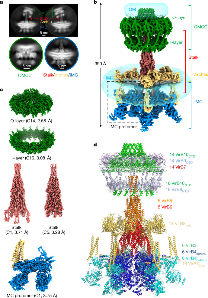
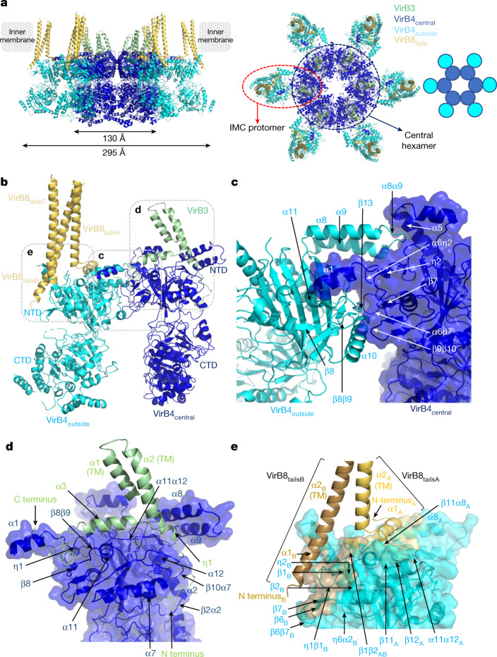
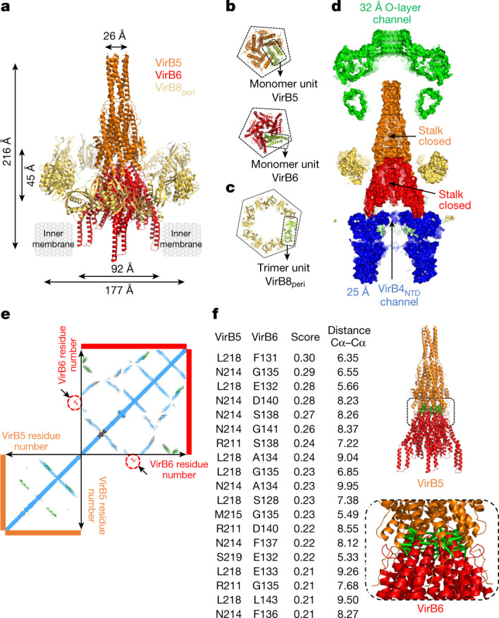
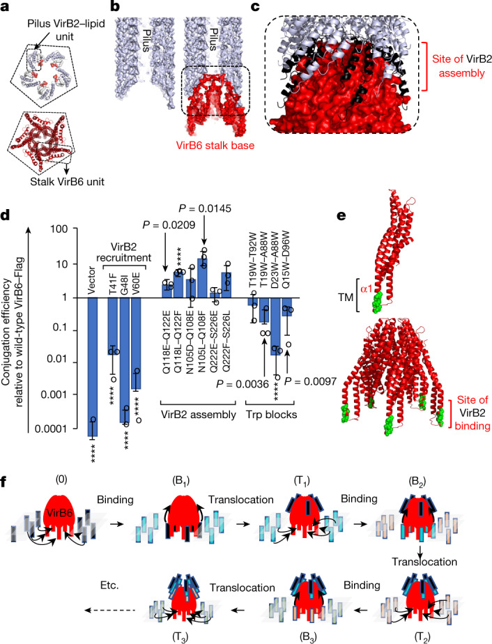
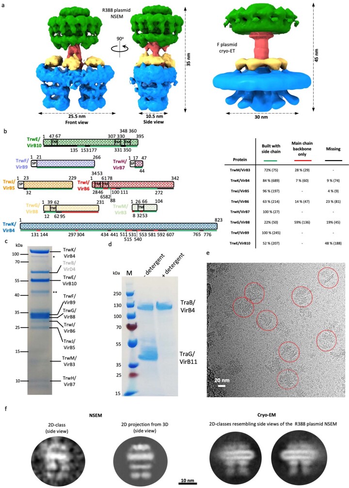
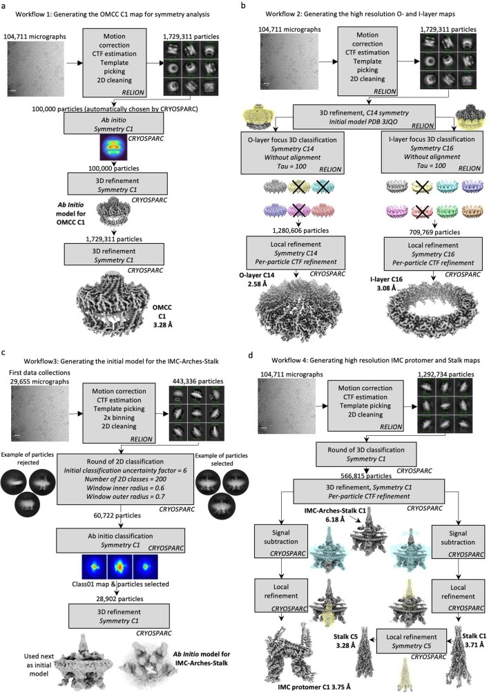
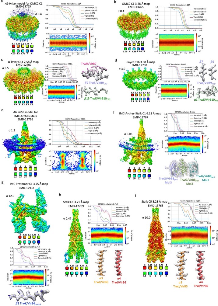
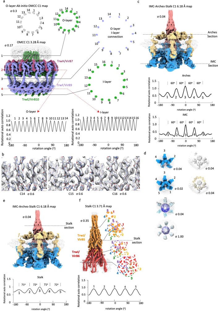
Bacterial conjugation is the fundamental process of unidirectional transfer of DNAs, often plasmid DNAs, from a donor cell to a recipient cell¹. It is the primary means by which antibiotic resistance genes spread among bacterial populations^2,3. In Gram-negative bacteria, conjugation is mediated by a large transport apparatus-the conjugative type IV secretion system (T4SS)-produced by the donor cell and embedded in both its outer and inner membranes. The T4SS also elaborates a long extracellular filament-the conjugative pilus-that is essential for DNA transfer^4,5. Here we present a high-resolution cryo-electron microscopy (cryo-EM) structure of a 2.8 megadalton T4SS complex composed of 92 polypeptides representing 8 of the 10 essential T4SS components involved in pilus biogenesis. We added the two remaining components to the structural model using co-evolution analysis of protein interfaces, to enable the reconstitution of the entire system including the pilus. This structure describes the exceptionally large protein-protein interaction network required to assemble the many components that constitute a T4SS and provides insights on the unique mechanism by which they elaborate pili.

Fig. 1. Overall structure of the R388 conjugative T4SS.

a, Representative 2D class averages of the T4SS obtained using cryoSPARC. Top, two 2D class averages of the entire T4SS demonstrate substantial flexibility of the OMCC relative to the stalk and the IMC. As a result, particles were subsequently centred on the OMCC (bottom left) or on the IMC–stalk (bottom right) and processed separately. b, Composite electron density map of the R388 T4SS. This map results from the assembly of two C1 maps, that of the OMCC (OMCC C1 3.28 Å map) and that of the IMC, arches and stalk (IMC–arches–stalk C1 6.18 Å map). The OMCC, stalk, arches and IMC are shown in green, red, yellow and dark blue, respectively, except for the VirB8_tails that are part of the IMC, which are shown in yellow. The various regions are labelled accordingly. σ levels for these maps are as in Extended Data Fig. 3b,f. For the detergent and/or lipid densities (in transparent light blue) at the membrane and outer membranes, the maps are shown at increased contour levels of 0.03 and 0.15, respectively, and smoothed using a Gaussian filter. c, Near-atomic resolution maps used in this study. Each map is labelled and contoured as in Extended Data Fig. 3. The resolution of the map is indicated. d, Overall composite model of the R388 T4SS. Each protein is in ribbon representation.

Fig. 2. Molecular details of IMC protein structures and interactions.

a, Overall structure of the IMC. The IMC is shown in ribbon representation, with subunits coloured dark blue (VirB4_central), cyan (VirB4_outside), pale green (VirB3) and yellow (VirB8_tails). Left, side view of the IMC. The external dimensions of the central VirB4 hexamer and of the IMC are indicated, as well as the position of the inner membrane derived from the density. Right, top view of the IMC. The IMC protomer and the central hexamer are shown in a dashed red oval and dark blue circle, respectively. A schematic diagram of the hexamer of VirB4 dimers is shown on the right. b, Overall structure of the IMC protomer. Proteins are shown and colour-coded as in a. The boxes locate the regions detailed in c–e. c, Details of the interactions between subunits within the VirB4 dimer. VirB4_central is shown in ribbon and semi-transparent surface in dark blue and VirB4_outside is shown in cyan ribbon. All secondary structures involved in the interactions are shown. d, Details of the interactions between VirB4 and VirB3. VirB4_central is shown in dark blue ribbon and surface representation and VirB3 is shown in pale green ribbon. All secondary structures containing residues involved in the interaction are labelled. e, Details of the interactions between VirB4_outside and two of the VirB8_tails. Only two are shown because although three VirB8_tails form a three-helix bundle, one of the helices makes very few interactions with VirB4_outside. The two VirB8_tails (VirB8_tailsA and VirB8_tailsB) are shown in yellow and wheat ribbons, respectively. VirB4_outside is shown in cyan ribbon and its semi-transparent surface is coloured yellow or wheat according to the VirB8_tail that it interacts with, or cyan for non-interacting surfaces.

Fig. 3. Molecular details of stalk and arches protein structures and interactions, and structure validation by co-evolution analysis.

a, Overall structure of the stalk and arches. Stalk and arches proteins are shown in ribbon coloured orange (VirB5), red (VirB6) and yellow (VirB8_peri). Proteins constituting the complexes and the dimensions of the two sub-complexes—stalk and arches—are indicated. b, Symmetry arrangements of VirB5 and VirB6. All proteins are shown in ribbon representation, colour-coded as in a, except one monomer in each box is shown in green. Top, bottom view of the VirB5 pentamer. Bottom, bottom view of the VirB6 pentamer. The dashed line in both illustrates the pentameric nature of each structure. c, Top view of the arches, showing the symmetry arrangement of VirB8_peri. All proteins are shown in ribbon representation. The arches are made of six trimeric units of VirB8_peri, one of which is shown in pale green and outlined; the rest are colour-coded as in a. The hexagon surrounding the hexamer of trimer highlights the six-fold symmetrical arrangement of this part of the structure. d, Cross-section of the T4SS surface. The channels are shown with dimensions of interest. The VirB4_outside subunits are not shown. e, Co-evolution at the interface of VirB5 and VirB6. Results of computational analysis. Each dot represents a pair of co-evolving residues with TrRosetta score ≥0.21. Dots are coloured blue (intra-protein co-evolution pairs), green (homo-oligomeric co-evolution pairs) or red surrounded by red circles and located by arrows (hetero-oligomeric co-evolution pairs). f, Co-evolution at the interface of VirB5 and VirB6. Left, list of hetero-oligomeric co-evolution pairs with TrRosetta scores above the threshold of 70% (Methods and main text) and Cα–Cα distances in angstrom in the structure reported here. Numbering is that of the R388 proteins. Full list in Supplementary Table 4. Right, mapping of co-evolution pairs listed in the table onto the VirB5–VirB6 stalk sub-complex structure. Pairs of residues across the interface are linked by green bars.

Fig. 4. Mechanism of pilus biogenesis by conjugative T4SSs.

a, Conjugative pili and the stalk have the same C5 symmetry. Top, the F pilus pentamer unit with TraA (VirB2) shown in white ribbon and the phospholipid shown in ball-and-stick representation colour-coded by atoms. Bottom, the VirB6 pentamer shown in red ribbon. A pentagon is shown to highlight the C5 symmetry. The outlines indicate the monomeric unit. b, Cut-away surface of the conjugative pilus (left) and of the pilus–VirB6 interaction (right). The pilus and VirB6 are shown in white and red surfaces, respectively. The outlined region is magnified further in c. c, Magnified view of the pilus–VirB6 interface. VirB6 is shown in red surface representation. The pilus VirB2 subunits are shown in white ribbon, except for the VirB2 pentamer at the bottom of the pilus, which is shown in black. The VirB2-contacting region on VirB6 defines this region as the site of VirB2 assembly (labelled). d, Mutational analysis of the surfaces of VirB6 hypothesized to form the binding/recruitment site (VirB2 recruitment), the assembly site (VirB2 assembly) and the effect of Trp mutations (Trp blocks) between the two sites. Locations of mutations in the structure are shown in Extended Data Fig. 10f,g. Conjugation results (data points indicated by open circles) are reported from three independent experiments (n = 3) and expressed as mean ± s.d. Unpaired two-tailed Student’s t-test with 95% confidence level was used to compare wild-type and mutant constructs. Significant P-values (less than 0.1) are shown, except where P ≤ 0.0001 (indicated by ****). e, Identification of the VirB2 binding/recruitment site on VirB6. The residues of VirB6 in the 50 top-scoring co-evolving residues obtained by TrRosetta between VirB2 and VirB6 were mapped onto the VirB6 structure (list in Supplementary Table 4). VirB6 is shown in red ribbon, except for the mapped residues, for which only the Cα atom is shown, coloured green. Top, the VirB6 monomer. Bottom, the VirB6 pentamer. f, Model of pilus biogenesis by conjugative T4SSs. Three cycles of VirB2 subunit incorporation are shown. VirB6 is shown as a dome-like red diagram with five legs (its transmembrane helices). The inner membrane is shown as semi-transparent lozenges. VirB2 subunits are shown as vertical rectangles colour-coded differently for each cycle. State 0 represents the structure described here. B_x, VirB2-bound state at the VirB6 transmembrane regions in cycle x. T_x, translocated state in cycle x in which the VirB2 subunits have reached the assembly site. Source data

Extended Data Fig. 1. Prior knowledge of conjugative T4SS architectures and proteins, purification and cryo-EM analysis of the R388 T4SS.

a, Known 3D architectures of conjugative T4SSs. Left and middle: front and side views of the low resolution negative-stained EM structure of the R388 T4SS (EMD-2567). Right: low resolution cryo-electron tomography structure of the F T4SS (EMD-9344 and EMD-9347). The IMC, Stalk, Arches, and OMCC are colour-coded as in Fig. 1b. b, Primary structure of the Trw/VirB proteins observed in this study. Each protein is named TrwX/VirBX according to convention where the first name is that of the Trw protein in the trw R388 plasmid gene cluster, and the second name is the name of its homologue in the Agrobacterium system. Each protein is shown as a hashed rectangle, the length of which is proportional to the length of its sequence. Colour-coding for each protein is as in Fig. 1d. Transmembrane segments as observed in the structure are shown in boxes labelled “TM”. Signal sequences are shown in empty boxes labelled SP. Lines under the rectangles indicate the parts of the sequence for which the electron density was of high enough quality to build a complete atomic model including side chains (in green), or where the secondary structures definition was good enough to build main chain secondary structures but not side chains (in red), or was so poor that no model could be built (in black). Boundary residue numbering for each box and line are indicated. Table at right recapitulates, for each protein, the proportion of the sequence either built with side chains, or with built main chain only, or missing in our structure. c, SDS-PAGE analysis of the purified R388 T4SS (For gel source data, see Supplementary Fig. 1a and corresponding legend in SI guide; n = 9 independent experiments). Molecular weight markers are indicated on the left. The proteins bands (identified by mass spectrometry) are labelled on the right. * and ** indicate minor contaminants (OmpA and OmpC). We purified a T4SS complex as in Redzej et al. (2017) i.e. a complex composed of 9 of the essential Trw/VirB proteins, TrwM/VirB3-TrwE/VirB10 and TrwB/VirD4 (Extended Data Fig. 1c), except that 1- the His-tag column purification step to enrich the preparation with VirD4-bound complexes was not carried out, 2- the complex was not crosslinked, a step shown by Redzej et al. (2017) to be required to keep TrwB/VirD4 bound, 3- concentration of the complex was achieved using ultracentrifugation, and 4- potential aggregates resulting from concentration were separated using sucrose density gradient centrifugation (see Methods). TrwB/VirD4 was therefore absent from the structure as it needs crosslinking to remain bound. Association of VirD4 with the T4SS may need stabilising through its interaction with the DNA substrate or its dissociation might be triggered by the cryogenic conditions. TrwD/VirB11 was also not part of the complex since it dissociates in the presence of detergents (Extended Data Fig. 1d). As a result, the structure contains TrwM/VirB3-TrwE/VirB10, a complex which was previously examined by negative stain EM (NSEM) by Low et al. (2014) and found to adopt the double-barrelled architecture. However, the purification protocol used to purify the complex here was greatly modified compared to that used in Low et al. (2014). Crucial to the improved conditions used here was the use of TDAO, a zwitterionic detergent. Moreover, concentration and separation from aggregates were also changed: in Low et al. (2014), the complex could not be concentrated without heavily aggregating, while here, due to a change in detergents mix, concentration using ultra-centrifugation was achieved as well as removing of minority aggregates by sucrose density gradient centrifugation. As a result of these significant modifications in the purification protocol, the yields were greatly improved (assessed to being between 20-30-fold), the complex being also much less prone to aggregation. Improved yields and higher quality sample combined to make the determination of this complex structure by cryo-EM possible. As explained in main text, a minority of particles in the cryo-EM data set presented here display the typical side views of the double-barrelled structure, indicating that the majority hexamer of dimers architecture we observe here must have been unstable in the buffer and NSEM conditions used by Low et al. (2014) since they did not observe it. In contrast, yields and stability of the double-barrelled complex obtained by Low et al. (2014) were low, making it impossible to solve its cryo-EM structure. d, SDS-PAGE analysis of the purified TraB/VirB4-TraG/VirB11 complex in the absence (No detergent) or presence of the detergents used to extract the T4SS (+detergent). For gel source data, see Supplementary Fig. 1b and corresponding legend in SI guide. n=3 independent experiments. e, Cryo-EM micrograph of the R388 T4SS. Red circles indicate examples of particles. 104,711 such micrographs over 7 datasets were collected. f, 2D classes found in the cryo-EM data set that show a view similar to that of the side views of the double-barrelled architecture observed by Low et al. (2014). The double-barrelled structure is characterised by a unique side view shown in Extended Data Fig. 1a, middle panel. Therefore, we asked whether such side views could be found in the cryo-EM data set described here. Left: an example of side view 2D classes (labelled “2D-class”) typically found in the NSEM double-barrelled architecture data and a corresponding 2D projection from the NSEM double-barrelled map (labelled “2D projection from 3D”). Right: 2 examples of similar side views but in the cryo-EM data set presented here. These 2D classes were generated using 2D classification of the set of 1,292,734 particles mentioned in Extended Data Fig. 1i, and selected for their resemblance to the side-view projections shown at left, resulting in the final selection of about 4,838 particles, i.e. circa 0.3% of the data set.

Extended Data Fig. 2. Workflow used to determine the structure of the various T4SS sub-complexes.

a, Workflow used to generate the OMCC C1 Ab Initio and 3.28 Å map. These maps were used for symmetry analysis of the OMCC O-layer and I-layer. b, workflow used to generate the O-layer C14 2.48 Å map and the I-layer C16 3.08 Å map. These maps were used to build and refine the atomic O- and I-layer models, respectively. c, workflow used to generate the initial Ab Initio model for the IMC-Arches-Stalk map. d, workflow used to generate the IMC-Arches-Stalk C1 6.18 Å map which was used 1- to build the Arches model, 2- for symmetry analysis of the IMC, the Arches, and the Stalk, 3- to derive the IMC protomer C1 3.75 Å map (used to build the IMC protomer model), 4- to derive the Stalk C1 3.71 Å and the Stalk C5 3.28 Å maps (used to build the Stalk model).

Extended Data Fig. 3. Cryo-EM maps used in this study.

For each map, the density coloured by local resolution, the average resolution derived from Fourier Shell Correlation (FSC), the angular distribution and, for panels c,d,f-i, a representative region of the electron density map with the final model of the T4SS built in it (in stick representation colour-coded as in Fig. 1d) are shown. Local resolution was calculated using CRYOSPARC (FSC cut-off 0.5) and coloured as indicated in the scale below the map. For each map, FSC plots show curves for correlation between 2 independently refined half-maps with no mask (blue), spherical mask (green), loose mask (red), tight mask (cyan) and corrected (purple). Cut-off 0.143 (blue line) was used for resolution estimation. a, the Ab Initio model for the OMCC; b, the OMCC C1 3.28 Å map; c, the O-layer C14 2.58 Å map; d, the I-layer C16 3.08 Å map; e, the Ab Initio model for the IMC-Arches-Stalk; f, The IMC-Arches-Stalk C1 6.18 Å map; g, the IMC protomer C1 3.75 Å map; h, the Stalk C1 3.71 Å map and i, the Stalk C5 3.28 Å map. All maps are sharpened. Contour levels and EMD codes are indicated.

Extended Data Fig. 4. Symmetry analysis of the various T4SS sub-complexes.

a, Symmetry analysis of the OMCC C1 Ab Initio and 3.28 Å maps. Upper left: section of the Ab Initio OMCC C1 map. The section is taken through the helical trans-membrane region of the O-layer. Middle Left: the non-averaged and unsharpened C1 map of the OMCC determined at a resolution of 3.28 Å colour-coded as in Fig. 1d. The contour level is indicated. The three filled lines and two dashed arrows labelled 1 to 5 indicate where the map sections have been taken for analysis shown at right (filled lines) and at bottom (dashed lines in red). Right: three sections of the map shown at left, one for the O-layer, one for the O-layer/I-layer connection, and one for the I-layer. Bottom: IMAGIC rotational auto correlation analysis of sections 2 and 4, independently corroborating C14 and C16 symmetry for the O- and I-layer, respectively. b, I-layer symmetry test. Using the OMCC C1 3.28 Å map (Extended Data Fig. 3b) as reference, three maps were generated using local refinement with a mask encompassing the I-layer and applying either C14, C15, or C16 symmetry. Highest interpretability is observed when C16 is used. The contour levels are indicated. The final model is shown in stick representation color-coded by atoms (red, blue, and white for oxygen, nitrogen, and carbon, respectively). c, Symmetry analysis of the IMC and Arches. Left: IMC-Arches-Stalk C1 6.18 Å unsharpened map colour coded as in Fig. 1b. The contour level is indicated. Two dashed lines through the Arches and the IMC indicate where the map sections have been taken for further symmetry analysis using IMAGIC shown underneath. However, for the Arches section, the section contains both the Arches and the Stalk and therefore, the Stalk region of the section was excluded from the analysis. The symmetry analysis of the IMC shows 5 peaks separated by a ~60° angle indicating 5 IMC protomers organised along a hexagon. A 6^th protomer has very weak occupancy: correspondingly, a weak but visible 6^th peak is observed in the IMAGIC symmetry analysis. Similar conclusions can be drawn from the analysis of Arches symmetry. d, Further symmetry analysis of the IMC and Arches. Left panels from top to bottom: bottom view of the IMC-Arches-Stalk C1 6.18 Å map coloured in blue and contoured at 0.04 σ level; same map contoured at 0.02 σ level; IMC hexameric model fitted into the same map (now coloured in semi-transparent grey); IMC hexameric model fitted into the cryo-ET map of the F plasmid IMC (EMD-9347 coloured in semi-transparent grey and contoured at 1 σ level; fitting correlation = 0.78). Right panels from top to bottom: section of the Arches and stalk density (0.04 σ level) in the IMC-Arches-Stalk C1 6.18 Å map coloured in semi-transparent grey; fit of the hexameric Arches into the external ring density. e, Symmetry analysis of the Stalk region in the unsharpened IMC-Arches-Stalk C1 6.18 Å map. The dashed line through the Stalk (in red) indicates where the map section has been taken for the symmetry analysis using IMAGIC shown underneath. Regularly spaced peaks spaced by a circa 72° are observed indicating C5 symmetry. f, Symmetry analysis of the non-averaged and unsharpened Stalk C1 3.71 Å map (colour coded orange for TrwJ/VirB5, red for TrwI/VirB6). The four lines indicate where the map slabs/slices shown at right have been taken. At right: four sections of the map shown at left, two for the TrwJ/VirB5 Stalk tip, one for the TrwI/VirB6 Stalk base and one in the middle. For one section, the symmetry analysis using IMAGIC is shown in the lower panel.

Extended Data Fig. 5. Generating the composite T4SS model shown in Fig. 1d.

a, Derivation of the C6 symmetry operators. The same particles used to generate the Ab Initio model for the IMC, Arches, and Stalk (Extended Data Fig. 2c) were used to generate an Ab Initio model with C6 symmetry imposed. The resulting map was used to generate the C6 symmetry operators using PHENIX. b, Positioning the OMCC relative to the IMC, Arches, and Stalk. As explained in Methods, the same C6 map was used to position the I-layer part of the OMCC. c, Verifying the positioning of the OMCC relative to the IMC, Arches and Stalk. While in most 2D classes, the OMCC is not aligned with the IMC-Arches-Stalk, in about 2.4 % of the particles, it is. Using these 2D classes, the distance (reported here) between the Arches and the I-layer was used to check that the positioning of the OMCC relative to the rest of the structure is correct.

Extended Data Fig. 6. Structural details of TrwK/VirB4_unbound and T4SS TrwK/VirB4 and IMC protomer.

a and b, Assessment of map resolution and quality for the TrwK/VirB4_unbound dimer (a) and trimer of dimers (b) structures. The local resolution variations of the corresponding map (left), the overall resolution derived from Fourier Shell Correlation (FSC) (upper right), the angular distribution (middle right) and a representative region of the electron density map with the final model of the TrwK/VirB4_unbound model built in it (lower right) are shown. Local resolution was calculated using CRYOSPARC and coloured as indicated in the scale below the map. The FSC plot shows curves for correlation between 2 independently refined half-maps with no mask (blue), spherical mask (green), loose mask (red), tight mask (cyan) and corrected (purple). Cut-off 0.143 (blue line) was used for average resolution estimation. The final model in representative regions of the maps is shown in magenta stick and ribbon representation for the dimer and trimer of dimers, respectively. c, Secondary structure definition of TrwK/VirB4 (Left), TrwM/VirB3 (Middle) and TrwG/VirB8_tails (right). The ribbon for each protein is coloured in rainbow colours from dark blue for the N-terminus to red for the C-terminus. All secondary structures are labelled. The IM is shown as a grey rectangle. d, Superposition of TrwK/VirB4_central and TrwK/VirB4_outside subunits of the IMC protomer. The two structures are very similar (RMSD in Cα position of 1.6 Å). Regions of differences between the two structures are indicated. e, Details of the interactions between two adjacent TrwK/VirB4_central subunits within the central hexamer. The two subunits are both shown in ribbon but coloured dark and sky blue, respectively. All secondary structures involved in the interaction are shown. Without the structure of ATP-bound TrwK/VirB4, it is unclear whether the TrwK/VirB4_central hexamer is in an active form or conformational changes are required to transition into one. f, Superposition of the TrwK/VirB4 dimeric unit of the T4SS (TrwK/VirB4_central and TrwK/VirB4_outside in blue and cyan, respectively, as in Fig. 2) onto the dimeric unit of TrwK/VirB4_unbound (in magenta and pink). These two structures superimpose very well with an RMSD in Cα position of 1.2 Å. g, Assembly of TrwK/VirB4_unbound. In TrwK/VirB4_unbound, three dimer units (shown here in magenta and pink, one of which is surrounded by a rectangle) come together in a roughly head to tail manner to form a trimer of dimers. Left: top view of the trimer of dimers structure. Right: schematic diagram showing the trimer of dimers configuration of TrwK/VirB4_unbound. h, Superposition of the TrwK/VirB4_unbound trimer of dimers (in magenta and pink) and the T4SS TrwK/VirB4 hexamer of dimers (in grey except for the TrwK/VirB4 dimer used for superposition which is shown in cyan and blue for TrwK/VirB4_outside and TrwK/VirB4_central, respectively). Left: the two types of assembly are superposed using the superposed dimeric units shown in panel f as a guide. In this superposition, the TrwK/VirB4_unbound trimer of dimers can be observed in an off-centered position relative to the T4SS TrwK/VirB4 hexamer of dimers. Right: two of the TrwK/VirB4_unbound trimers of dimers superposed on two diametrically opposite TrwK/VirB4_central-TrwK/VirB4_outside dimers results in a double-barrelled architecture reminiscent of that observed in the NSEM double-barrelled structure by Low et al. (2014) where two off-centered barrels (also trimers of dimers) were observed side by side as shown in Extended Data Fig. 1a, left panel. i, Docking of two TrwK/VirB4_unbound trimers of dimers (green and blue ribbons) into the NSEM double-barrelled structure. Left: NSEM map of the T4SS double-barrelled architecture contoured at σ 10 (EMD-2567). The region corresponding to TrwK/VirB4 is within the middle and lower tiers densities of each barrel (see Low et al. (2014) for details). The two dashed arrows indicate where the sections shown at right have been taken. The TrwK/VirB4_unbound NTDs fit well into the middle tier density (fitting correlation 0.59; upper right panel) while the CTDs, which are very flexible because of being unconstrained, protrude out of the lower tier density (fitting correlation 0.29; lower right panel).

Extended Data Fig. 7. Details of Stalk and Arches proteins.

a, Secondary structure definition of TrwI/VirB6 (left), TrwJ/VirB5 (middle) and TrwG/VirB8_peri (right). The ribbon for each protein is coloured in rainbow colours from dark blue for the N-terminus to red for the C-terminus. All secondary structures are labelled. b, Locations of the predicted hydrophobic TMs in TrwI/VirB6. The TMpred server suggests a number of potential TMs in TrwI/VirB6: these predicted TMs are here mapped in white onto the TrwI/VirB6 structure. Of these, only two are observed inserting in the inner membrane, α1 and α2. All α-helices that contain a hydrophobic region are labelled. Boundary residues for these regions and location of the TM region are indicated. Also, we observe that the region of the IM within the TrwI/VirB6 pentamer is disrupted while it remains intact outside it (indicated in the figure). c, Interactions between subunits within the TrwI/VirB6 pentamer. Two adjacent subunits are shown in pink and red ribbon, respectively. Interface residues in the subunit in red are shown as surface coloured in grey. All secondary structures where residues are involved in interactions are labelled. The positions of the TMs as defined in the electron density map are shown. d, Interactions between subunits within the TrwJ/VirB5 pentamer. Two adjacent subunits are shown in orange and yellow ribbon, respectively. Interface residues in the subunit in orange are shown in surface representation coloured in orange. All secondary structures where residues are involved in interactions are labelled. e, Superposition of TrwJ/VirB5 with two known VirB5 homologues and one pore-forming protein Hemolysin E. Left: superposition with TraC (PDB entry code: 1R8I), the VirB5 homologue of the pKM101 plasmid-encoded T4SS. Middle: superposition with CagL (PDB entry code: 3ZCI), the VirB5 homologue in the Cag pathogenicity island of Helicobacter pylori. Right: superposition with Hemolysin E (PDB entry code: 6MRU), a bacterial pore-forming protein, one of top hits in DALI. The superposition is particularly good with the C-terminal half of CagL and Hemolysin E (RMSD of 3.1 and 3.2 Å in Cα atoms, respectively). f, Interactions between TrwJ/VirB5 and TrwI/VirB6. One TrwJ/VirB5 subunit (in orange ribbon) interacts with two TrwI/VirB6 subunits (shown in red and pink). For TrwI/VirB6, the regions of two subunits involved in interactions with TrwJ/VirB5 are shown as a surface while the rest of the molecules are shown in ribbon. Secondary structures contributing residues to the interfaces are labelled. g, Interactions between subunits within the TrwG/VirB8_peri homo-trimeric unit. Left: the homo-trimeric TrwG/VirB8_peri unit. Each subunit is shown in a different colour, pale cyan (MolC), pale green (MolB) and pale blue (MolA), respectively. Centre: the VirB8_peri dimer from H. pylori (PDB entry code: 6IQT). The orientation shown results from a superposition of this dimer on MolA/MolB of TrwG/VirB8_peri. As can be seen, the interface between subunits within this dimer is similar to that of the MolA/MolB interface between TrwG/VirB8_peri subunits. Right: the VirB8_peri dimer from Brucella suis (PDB entry code: 2BHM). The orientation shown results from a superposition of this dimer on MolB/MolC of TrwG/VirB8_peri. As can be seen, the interface between subunits within this dimer is similar to that of the MolB/MolC interface between TrwG/VirB8_peri subunits. RMSDs are reported in main text. Secondary structures contributing residues to the interfaces are labelled. h, Interface between TrwG/VirB8_peri trimeric units in the Arches hexamer. In the T4SS structure presented here, six trimeric units come together to form the Arches. Inset: top view of the TrwG/VirB8_peri trimeric units forming the Arches hexamer. The dashed lined box locates the region zoomed-in at right. One trimeric unit is colour-coded as in panel g, while the adjacent trimeric units are coloured in yellow orange. The secondary structures involved in interactions between trimeric units are labelled.

Extended Data Fig. 8. Details of the OMCC proteins and description of extra-densities that could not be ascribed.

a, Structure of the O-layer and I-layer. All proteins are in ribbon, with TrwH/VirB7, TrwF/VirB9 and TrwE/VirB10 shown in magenta, light blue and green, respectively. Dimensions of interest are reported. Proteins constituting the shown complexes are indicated. Upper left: side view of the O-layer. Upper right: top view of the O-layer. Lower left: side view of the I-layer. Lower right: top view of the I-layer. b, Secondary structure definition of TrwE/VirB10_CTD (left), TrwF/VirB9_CTD (middle) and TrwH/VirB7 (right). The ribbon for each protein is coloured in rainbow colours from dark blue for the N-terminus to red for the C-terminus. All secondary structures are labelled. Note that loop between α3 and α4 of TrwE/VirB10_CTD is disordered and, as a result, these helices appear to insert half-way through the membrane. However, in Chandran et al. (2009), we showed that the loop connecting the two helices is accessible from the surface of the bacterium and therefore completes the TM region and emerges out to the bacterial cell surface. c, Superposition of the structures of the hetero-trimeric unit of the O-layer from pKM101 (grey) and R388 (light blue, green and magenta for TrwE/VirB10_CTD, TrwF/VirB9_CTD, and TrwH/VirB7, respectively). The two heterotrimers superimpose with an RMSD in Cα of 0.8 Å. The various parts of the heterotrimeric complex are shown and labelled. d, Superposition of the structure of the hetero-dimeric unit of the I-layer from R388 (TrwF/VirB9_NTD (light blue) bound to α1 of TrwE/VirB10_NTD (green)) and that of the same region of the Xanthomonas citri I-layer (grey). The two structures superimpose with an RMSD in Cα of 0.9 Å. e, The interfaces between TrwF/VirB9_NTD subunits (upper panel; the domain is in rainbow colour from N- to C-terminus) and between α1 of TrwE/VirB10_NTD and two TrwF/VirB9_NTD (lower panel). Secondary structures contributing residues to the interfaces are labelled. f, Insertion of two additional TrwF/VirB9_NTD-α1TrwE/VirB10_NTD complexes diametrically opposite within the I-layer. Left: the OMCC C1 3.28 Å map shown in grey with TrwF/VirB9 linkers between the O- and I-layers shown in purple (0.17 σ level). Dashed line box indicates the section of density shown at right. Right: top view of the I-layer map section indicated by the dashed line box at left. The two inserted TrwF/VirB9_NTD domains are recognizable because they do not have the linker connecting their NTDs (I-layer) to their CTDs (O-layer). g, Interactions between TrwI/VirB6 (the base of the Stalk) with TrwM/VirB3 and TrwK/VirB4 (in the IMC). TrwM/VirB3 and TrwI/VirB6 are shown in pale green and red ribbon, respectively, while two central TrwK/VirB4 subunits are shown in dark blue and sky blue ribbon and semi-transparent surface. Secondary structures contributing interacting residues are labelled. Inset: overview of the location of the zoomed-up structure shown in main panel. h, Additional densities (shown in semi-transparent grey) observed in the Arches and the IMC potentially corresponding to a fourth molecule of TrwG/VirB8. Additional density in the IMC-Arches-Stalk C1 6.18 Å map (Extended Data Fig. 3f) was observed forming a helix tube bound to the 3-helices bundle of the TrwG/VirB8_tails. Correspondingly, an additional density was observed near the TrwG/VirB8_peri ring. This may indicate the presence of a fourth TrwG/VirB8 subunit (shown in magenta ribbon). Finally, there is density between the TrwG/VirB8_tails and the TrwG/VirB8_peri domains, which we hypothesize might be formed by the residues in between the two domains (residues 62-95; Extended Data Fig. 1b). However, the densities were too poor to be assigned and we remain unsure as to potential interpretations and assignments. i, Extra density also observed in the IMC-Arches-Stalk C1 6.18 Å map (Extended Data Fig. 3f). Left: overall structure of the T4SS with a dashed lined box showing the location of the extra density. Proteins are colour-coded as in Fig. 1d and are in ribbon representation, except for TrwE/VirB10 which is in surface representation. Right: zoom-in on the region of the structure shown in the dashed lined box shown at left. Two extra densities (in green) are seen at σ 0.04 which merge into one at σ 0.02. These indicate a structure that makes contact with TrwG/VirB8_peri and that is flexibly (shown in dashed lines) connected to another structure that makes contact with the TrwI/VirB6 TM helices and with the two subunits of the TrwK/VirB4 dimer. The density was too poor to be assigned but could correspond to TrwE/VirB10_NTD, which is known to not only make a major part of the OMCC but also has an IM TM and a cytoplasmic tail that, in other T4SSs, has been known to interact with VirB8, VirB6 and VirB4^–. However, it could be that this stretch of density may correspond to different proteins.

Extended Data Fig. 9. Validation of the T4SS heterologous interfaces using the co-evolution method as implemented by TrROSETTA.

For each panel, three sub-panels are shown. Upper panel: plots of pairwise TrROSETTA contact probability score. Each dot represents a pair of co-evolving residues with TrROSETTA score larger than a case-specific threshold (see Methods). Dots are coloured blue, green, or red (also surrounded by a red dashed line), for intra-protein co-evolution pairs, homo-oligomeric co-evolution pairs, and hetero-oligomeric co-evolution pairs, respectively. Lower panels: mapping of top co-evolution pairs onto the structure reported here (70% threshold except for the TrwK/VirB4_central - TrwM/VirB3 interaction where the 30 top pairs are mapped; in green in Supplementary Table 4). Dashed box in lower left panel locates the structure showed right. Pairs of residues across the interface are linked by red bars. As can be seen from the list in Supplementary Table 4, going down the list, distances greater than the generally accepted 12 Å limit for Cα-Cα distances between interface residues^, are found but rank very poorly (pairs in yellow in Supplementary Table 4). a, Plot and mapping of co-evolving residue pairs between TrwK/VirB4_central and TrwM/VirB3. b, Plot and mapping of co-evolving residue pairs between TrwE/VirB10_CTD and TrwF/VirB9_CTD in the OMCC O-layer. c, Plot and mapping of co-evolving residue pairs between TrwK/VirB4_outside and TrwG/VirB8_tails. See details in Supplementary Table 4 and Methods. Note that residues of TrwK/VirB4_outside that interact with α1 residues in TrwG/VirB8_tailsA (α1A in Fig. 2e) were not among the top 100 co-evolving residue pairs between these two proteins (Supplementary Table 4), therefore this very small part of our structural model remains unvalidated.

Extended Data Fig. 10. Validation of the VirB4-VirB11 interaction, mutational analysis of the VirB2-binding and -assembly sites on VirB6, and conformational changes required or not required for the pilus to pass through the Arches (not required), the I-layer (not required) and the O-layer (required).

a, Assessment of the TraB/VirB4 and TraG/VirB11 ALPHAFOLD models against known individual structural homologues. Left: superposition of the ALPHAFOLD model of TraB/VirB4 (in yellow) with the cryo-EM model of TrwK/VirB4_central (in dark blue; this work). Right: superposition of the ALPHAFOLD model of TraG/VirB11 (in yellow) with the crystal structure of B. suis VirB11 (2GZA, in magenta). RMSD in Cα position are 1.26 Å and 1.23 Å, respectively. b, The VirB4-VirB11 structural model and the two independent methods used for its validation. Left: ALPHAFOLD structure of a complex of TraB/VirB4 (dark blue ribbon) bound to TraG/VirB11 (magenta ribbon). Middle: first validation of the complex model using the mapping of the TrROSETTA top-scoring (70% threshold) co-evolving pairs (listed in green in Supplementary Table 4; see Methods). Right: location of the interface residues mutated to provide a second independent validation of the ALPHAFOLD complex model. c, Pull-down of the TraB/VirB4-TraG/VirB11 wild-type and mutated complexes. Pull-downs were performed by taking advantage of a His-Tag at the C-terminus of TraB/VirB4. Samples were loaded so as to equalise as much as possible the amount of TraB/VirB4. The coomassie-stained gel is shown in upper panel, while the Western blots using anti-His antibodies to detect TraB/VirB4 (middle panel) or anti-Strep antibodies to detect TraG/VirB11 (lower panel) are shown below. Mutants are indicated as well as the positions of some molecular markers (MW), and those of TraB/VirB4 and TraG/VirB11. All mutated proteins expressed as well as wild-type and were equally soluble (not shown). Although similar amounts of TraB/VirB4 are loaded, the TraG/VirB11 band is less intense in the mutants, indicating weaker interactions; moreover, the inability of interface mutants to bind TraG/VirB11 also results in a slight degradation of TraB/VirB4 which is not observed in the wild-type interaction. For gel source data, see Supplementary Fig. 1c and corresponding legend in SI guide. n = 3 independent experiments. d, PATCHDOCK docking of the TraA/VirB2 and the TrwI/VirB6 pentamers. The docking is based on shape complementarity. The top-scoring model is shown in ribbon representation colour-coded black and red for TraA/VirB2 and TrwI/VirB6, respectively. The TrROSETTA analysis of VirB2-VirB6 did not detect any pairs involving VirB6 residues in this putative assembly site. This is not surprising: transient interactions are known to provide only weak co-evolutionary pressure and one indeed expects VirB2 subunits to make only transient and weak interactions with the assembly site so as to not prevent incoming VirB2 subunits from displacing already assembled subunits at the base of the pilus. e, Model of the T4SS with bound F pilus and ALPHAFOLD TrwD/VirB11 model. Proteins are shown in ribbon colour-coded as in Fig. 1d, with the pilus in blue-white and TrwD/VirB11 in magenta. The O-layer is in the open conformation as shown in panel k. f, Overall view of the TrwI/VirB6 residues mutated in this study. Inset at left: overall stalk view in red (TrwI/VirB6) and orange (TrwJ/VirB5) ribbon representation. The dashed line box indicates the zoomed-in region at right. Residues mutated are shown in ball-and-stick representation. Mutations increasing conjugation are shown in green while those decreasing conjugation are shown in blue. The sites are labelled. For the VirB2- binding/recruitment site (labelled “recruitment site”), residues were mutated to bulky residues (T41F or G48I) or to acidic residue (V60E), all three anticipated to interfere with VirB2-binding. For the VirB2-assembly site, 3 pairs of double mutations, one to acidic residues, the other to hydrophobic, were designed with the intention of potentially increasing the affinity of the site for VirB2 subunits, thereby potentially increasing the binding of the pilus to its base. The R388 and pKM01 pilus are known to only weakly attach to the cell surface and thus, mutations increasing its affinity to its VirB6 base might increase its residency time, thereby affecting conjugation. Note that none of the mutants in the assembly site overlaps with the TrwJ/VirB5 binding site. Finally, For the Trp-blocks, 3 double mutations to W were implemented, with the intention to create obstacles preventing VirB2 subunits from reaching the assembly site while translocating from their binding site. g, Details of residues mutated in the assembly site (left), the recruitment/binding site (middle) and to generate the Trp blocks (right). Residues and TrwI/VirB6 are as in panel e. Residues are labelled. h, Western blot analysis of wild-type and mutated TrwI/VirB6 in the membrane (see Methods). All mutated TrwI/VirB6 proteins express similarly and all locate to the IM to the same extent as wild-type. Note that Redzej et al. (2017) have shown that deletion of TrwI/VirB6 does not affect the integrity of the T4SS except for TrwJ/VirB5 which is lost. However, none of the mutations described here are within the TrwI/VirB5 binding site and thus, we can safely conclude that the T4SS assembly is not affected in any of the mutants. For gel source data, see Supplementary Fig. 1d and corresponding legend in SI guide. n=3 independent experiments. i, Position of the VirB6 residues involved in the 50 top-scoring co-evolution pairs listed in Supplementary Table 4 for the VirB2/VirB6 interaction. All locate in the α1 helix, making this helix a strong candidate for VirB2 binding and recruitment. Inset at left: overall TrwI/VirB6 pentamer structure in red ribbon representation. Dashed line box indicates the zoomed-in region at right. The Cα atom of each residue is shown in sphere representation coloured in green. j, Position of the VirB3 residues involved in the 50 top-scoring co-evolution pairs listed in Supplementary Table 4 for the VirB2/VirB3 interaction. All locate in the α1 helix, making this helix another strong candidate for VirB2 binding. The Cα atom of each residue is shown in sphere representation coloured in blue white. k, Conformational change needed to open up the O-layer OM channel. As shown in Extended Data Fig. 8a, c, the heterotrimeric unit of the O-layer contains a 2-helix bundle that traverses the OM. 14 of these bundles form the OM channel. For the pilus to go across the OM through this OM channel, the 14 helical bundles need to open up, a conformational change that only requires a hinge motion along the two linkers that connect each of the helical bundles to the TrwE/VirB10_CTD β-barrel. Left panel: superposition of the heterotrimeric unit of the open (in green) and partially closed (in grey) O-layer. The partially closed state is that seen in the T4SS structure solved here. The open state is the one modelled here as described in Methods. Right panel: superposition of the entire open and partially closed O-layer states. The dimension of the open channel is shown. l, Cut-away of the structure with pilus shown in panel e. Colour-coding for the various proteins are indicated by labels, except for the pilus which is as in panel e. Left: cut-away at the level of the Arches. Middle: cut-away at the level of the I-layer. Right: cut-away at the level of the O-layer in its open conformation. These panels illustrate the fact that no conformational change is needed in the Arches or the I-layer for the pilus to pass through during pilus biogenesis but is needed to pass through the O-layer. We hypothesize that the Arches and the I-layer provide scaffolding rings through which the pilus is directed.

References

1. Waksman G. From conjugation to T4S systems in Gram-negative bacteria: a mechanistic biology perspective. EMBO Rep. 2019;20:e47012. - PMC - PubMed
1. Virolle C, Goldlust K, Djermoun S, Bigot S, Lesterlin C. Plasmid transfer by conjugation in Gram-negative bacteria: from the cellular to the community level. Genes. 2020;11:1239. - PMC - PubMed
1. Barlow M. What antimicrobial resistance has taught us about horizontal gene transfer. Methods Mol. Biol. 2009;532:397–411. - PubMed
1. Costa TR, et al. Secretion systems in Gram-negative bacteria: structural and mechanistic insights. Nat. Rev. Microbiol. 2015;13:343–359. - PubMed
1. Costa, T. R. D. et al. Type IV secretion systems: advances in structure, function, and activation. Mol. Microbiol.10.1111/mmi.14670 (2020). - PMC - PubMed