High-throughput total RNA sequencing in single cells using VASA-seq

Abstract

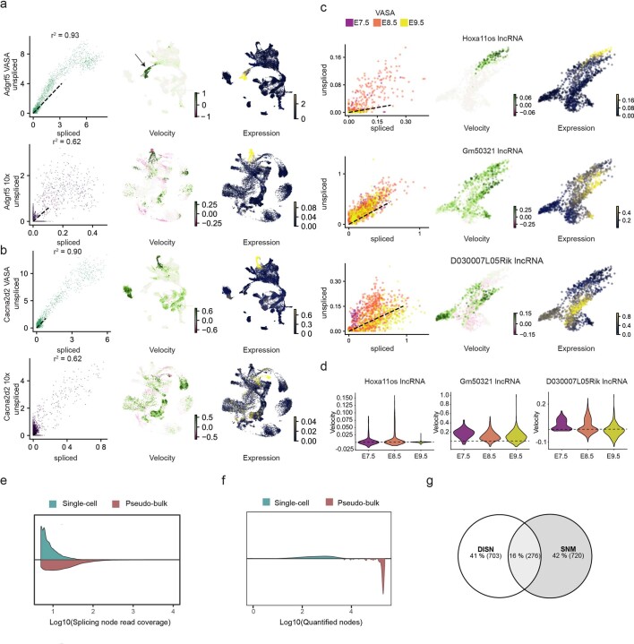
Most methods for single-cell transcriptome sequencing amplify the termini of polyadenylated transcripts, capturing only a small fraction of the total cellular transcriptome. This precludes the detection of many long non-coding, short non-coding and non-polyadenylated protein-coding transcripts and hinders alternative splicing analysis. We, therefore, developed VASA-seq to detect the total transcriptome in single cells, which is enabled by fragmenting and tailing all RNA molecules subsequent to cell lysis. The method is compatible with both plate-based formats and droplet microfluidics. We applied VASA-seq to more than 30,000 single cells in the developing mouse embryo during gastrulation and early organogenesis. Analyzing the dynamics of the total single-cell transcriptome, we discovered cell type markers, many based on non-coding RNA, and performed in vivo cell cycle analysis via detection of non-polyadenylated histone genes. RNA velocity characterization was improved, accurately retracing blood maturation trajectories. Moreover, our VASA-seq data provide a comprehensive analysis of alternative splicing during mammalian development, which highlighted substantial rearrangements during blood development and heart morphogenesis.

Fig. 1. Overview of the VASA-seq workflow and benchmarking against other state-of-the-art methodologies.

a, Overview of the VASA-seq single-cell molecular workflow. Single cells are lysed, and RNA is fragmented. Fragments are repaired and polyadenylated, followed by reverse transcription (RT) using barcoded oligo-dT primers. The cDNA is made double stranded and amplified using IVT. aRNA is depleted of rRNA, and libraries are finalized by ligation, RT and PCR, which leave fragments ready for sequencing. b, Picture illustrating the single-cell encapsulation process using droplet microfluidics. The single cells (green) are co-encapsulated with a barcoded bead (purple), lysis and fragmentation mix (blue), and compartmentalization is achieved with the addition of fluorinated surfactant oil (red) at the flow-focusing junction. c, Picture illustrating the picoinjection of reagents (green) to single-cell lysates (light blue/purple). The droplet surface tension is perturbed using an electric field that allows for the subsequent additions of end repair/poly(A) and RT mix. d, Cross-contamination test for VASA-drop was carried out using HEK293T cells (human) and mouse embryonic stem cells (mouse). Barcodes with more than 25% of detected UFIs belonging to the other species were considered doublets/mixed (red). Detected barcodes with low UFIs (<7,500) were discarded (gray). The remainder were assigned to either human (magenta) or mouse (blue). e, Gene body coverage comparison along protein-coding genes. VASA-seq showed even coverage, whereas 10x, Smart-seq-total and Smart-seq3 had a bias toward transcript termini (3′ or 5′ and 3′, respectively). f, The number of detected annotated genes in HEK293T cells, for each method, is plotted against the number of reads (after quality filtering, adapter removal and homopolymer trimming) per cell across different downsampling thresholds. The saturation curves showed that VASA-seq was the most sensitive of the methods. Curvature of gene detection indicated that full complexity was not reached for the method when 75,000 reads were allocated to each cell. Only cells that were sequenced to at least 75,000 reads were used (VASA-plate: n = 174, VASA-drop: n = 376, Smart-seq3: n = 113, Smart-seq-total = 260, 10x Chromium: n = 288).

Fig. 2. VASA-seq enables novel marker gene detection in the developing mouse embryo.

a, Schematic figure of mouse embryo morphology at developmental stages E6.5, E7.5, E8.5 and E9.5 (left to right). b, Fraction of transcripts per biotype in VASA-seq compared to 10x Chromium for mouse embryos at each timepoint using the 20% terminal portion of genes. The comparison includes protein-coding genes (top-left panel), lncRNAs (top-right panel), TFs (bottom-left panel) and sncRNAs (bottom-right panel). c, Percentage of genes detected in VASA-seq compared to 10x for each timepoint using the 20% terminal portion of genes. 70.8–76.2% of the detected genes were shared between the methods; 18.7–25.3% were detected only in VASA-seq; and 2.4–5.1% were detected only in 10x. d, Strategy to transfer cluster identity from 10x Chromium or VASA-seq (reference technology) to VASA-seq or 10x Chromium (target technology) at the single-cell level. First, for a given cluster in the reference technology, a background histogram of the distances between cells in that cluster and their corresponding first nearest neighbor in the target technology is obtained (gray arrows and gray histogram). Next, each cell in the target technology is assigned to the cluster of its nearest neighbor cell in the reference technology (black and green arrows) with a score equal to the area under the left curve resulting from the intersection between the cell–cell distance and the corresponding background histogram (dashed area). This procedure is then repeated for all clusters in the reference technology. e, UMAP of E8.5 mouse embryo cells from 10x Chromium (n = 9,358) and VASA-seq (n = 7,899) that were part of equivalent clusters using the 20% terminal portion of genes. Clusters that are detected in both technologies are marked with numbers 1–43, and each cluster is colored according to the cell type category: green, blood; blue, ectoderm; purple, endoderm; orange, mesoderm; gray, epiblast. Gray fill in cluster label indicates extra-embryonic contribution; black fill indicates embryonic contribution. f, Scatter plot showing the number of differentially expressed genes per cluster in VASA-seq (x axis) versus 10x Chromium (y axis) for spliced protein-coding genes (left panel), unspliced protein-coding genes (middle panel) and lncRNAs (right panel) using the 20% terminal portion of genes. Numbers indicate clusters where a higher number of marker genes were detected in 10x Chromium. Clusters are colored according to the cell type category: green, blood; blue, ectoderm; purple, endoderm; orange, mesoderm, gray, epiblast. g, Heat maps showing the ratio of differential upregulated genes (log₂ fold change >2 and P < 0.01), per cluster, between VASA-seq and 10x Chromium using the 20% terminal portion of genes. Columns display spliced protein-coding genes (left panel), unspliced protein-coding genes (middle panel) and lncRNAs (right panel), and rows are clusters. Red color indicates when marker genes are more predominantly detected in VASA-seq; blue color indicates when higher numbers of marker genes are detected in 10x Chromium. The statistical test used was a two-sided t-test, and P values were uncorrected for multiple comparisons. h, Examples of newly detected unspliced lncRNA marker genes in VASA-seq for E8.5: Foxl2os in paraxial mesoderm progenitors (left panel), AI115009 in mesenchyme (middle panel) and C130021I20Rik in forebrain/midbrain/hindbrain and surface ectoderm (right panel).

Fig. 3. Histone gene expression robustly identifies cycling cells.

a, Volcano plot showing differentially expressed genes between VASA-seq (right, positive values) and 10x Chromium (left, negative values). Genes that are always highly differentially expressed across timepoints and have a log₂ fold change >4 and P < 0.001 are colored; purple color indicates non-polyadenylated, and orange color indicates polyadenylated genes. Many of the differentially expressed genes enriched in the VASA-seq dataset are histone genes. The statistical test used was a two-sided t-test, using uncorrected P values for multiple comparisons. b, Histogram showing the distribution of histone gene expression in VASA-seq compared to 10x Chromium. The overlayed dashed black line shows a bimodal Weibull distribution, and the dashed red line shows a single Weibull distribution. c, Histogram showing the distribution of histone gene expression in VASA-seq labeled with the estimated cell cycle phase using the expression of S and G2M genes for scoring. Detected histone expression in S-phase does not correlate with predictive cell cycle estimation. d, Cells are identified as cycling/S-phase (blue) and non-cycling (yellow) based on the total histone gene expression shown in Fig. 3b. UMAP of the VASA-seq embryonic atlas before (left panel) and after (right panel) removal of cell cycle genes. e, Cell type annotated UMAP of the aggregated VASA-seq dataset after removal of cell cycle genes. Each color and number represent a cell type, called manually based on marker gene expression for each Leiden cluster. Smaller panels (right) highlight cells sampled at each timepoint (E6.5, E7.5, E8.5 and E9.5) in black. In total, 40 different cell types were identified: 1-erythropoiesis (expansive, S-phase), 2-somites, 3-paraxial mesoderm, 4-intermediate mesoderm I, 5-caudal epiblast, 6-lateral plate mesoderm/intermediate mesoderm primordium, 7-spinal cord (differentiated neurons), 8-endothelium, 9-preplacodal/placodal region, 10-rhombomeres (hindbrain), 11-forebrain/hindbrain (isthmus), 12-epiblast (E7.5), 13-forebrain, 14-spinal cord (differentiated neurons), 15-neural crest, 16-allantois, 17-cranial mesoderm, 18-lateral plate mesoderm, 19-early caudal epiblast, 20-trophectoderm, 21-dorsal surface ectoderm, 22-anterior neural crest, 23-pharyngeal arches, 24-primitive erythroid progenitors, 25-caudal epiblast (E7.5), 26-endoderm, 27-visceral endoderm, 28-first heart field, 29-myofibroblasts, 30-epiblast (E6.5), 31-spinal cord (cycling progenitors), 32-pharyngeal arches, 33-primitive heart tube, 34-outflow tract, 35-secondary heart field, 36-intermediate mesoderm I, 37-parietal endoderm, 38-pro-nephros, 39-mesodermal unknown and 40-node. f, Percentage of cycling/S-phase cells per cell type. Average number of cycling cells is 65% (black line) ± 11% (red dashed lines) across all cell types. Late primitive erythrocytes (green) diverge from the average by having 84% of the cells in S-phase. Node cells (brown) and primitive heart tube (pink) have much fewer cells in S-phase—20% and 30%, respectively. g, Plots showing the percentage of cells in S-phase per cell type that spans over three timepoints (E6.5–E8.5, left panel; E7.5–E9.5, right panel). Trophectoderm (light brown) had an unchanged pattern, whereas endothelium (green), allantois (pink), lateral plate mesoderm (blue), endoderm (light green), visceral endoderm (light blue) and outflow tract (dark pink) all had a decreasing fraction of cycling cells as time passes. Allantois has the biggest difference, with 38% cycling in E9.5 compared to 79% in E7.5. The points are the mean and standard error of the mean obtained by bootstrapping the percentage of cells in S-phase for each equivalent cluster and biotype 1,000 times. The number of cells were: n = 140, 32 for cluster 20 and 27 at timepoint E6.5, respectively; n = 105, 340, 314, 392, 156, 171 and 69 for clusters 8, 16, 18, 20, 26, 27 and 34 at E7.5, respectively; n = 810, 552, 331, 117, 284, 339 and 121 for clusters 8, 16, 18, 20, 26, 27 and 34 at E8.5, respectively; and n = 345, 78, 30, 117 and 71 for clusters 8, 16, 18, 26 and 34 at E9.5, respectively. h, Heatmap showing differentially expressed single annotated histone genes. Rows display genes, and columns display cell types. Cell type categories/germ layers can be identified by color above the heat map. i, Example of marker histone gene expression plotted on the UMAP; red represents high expression, and blue represents low expression. H2bc15 is highly expressed in most cell types but absent in certain cell types. H2bc1 is solely expressed in the early epiblast (E6.5, cell type 30), whereas H2bu2 is specific to the ectoderm germ layer and epiblasts (cell types 12 and 30).

Fig. 4. Increased intronic capture with VASA-seq improves RNA velocity measurements.

a, UMAP of all four timepoints for VASA-seq (E6.5–E9.5). Velocity is shown as arrows and each timepoint as a separate color. The black arrow indicates blood maturation trajectory. b, Violin plot of confidence values for VASA-seq in green (left panel) and 10x Chromium in dark purple (right panel). Only the equivalent E6.5, E7.5 and E8.5 timepoints are included in the comparison. Average RNA velocity confidence was 0.84 ± 0.12 (s.d.) for VASA-seq and 0.65 ± 0.12 (s.d.) for 10x. n number of cells were 21,497 (VASA-seq) and 16,945 (10x Genomics Chromium). Data in the box plot represent the 25%, median (center) and 75% percentiles with minimum and maximum values. c, Venn diagram showing the significant genes, according to the scVelo package, for VASA-seq and 10x Chromium. In all, we found 1,492 genes that were significant in both datasets, 1,069 that were significant only in VASA-seq and 26 that were significant only in 10x. d, Histograms showing goodness of fit (r²) for the 1,492 genes that were significant in both VASA-seq and 10x Chromium. Average values were 0.74 ± 0.18 (s.d.) for VASA-seq and 0.38 ± 0.25 (s.d.) for 10x Chromium. e, UMAP of the equivalent 10x Chromium dataset (E6.5, E7.5 and E8.5) after filtering. Velocity is shown as arrows and each timepoint as a separate color. The black arrow indicates blood maturation trajectory. f, Predicted latent time projected on the blood and erythroid progenitor subsets, showing incorrect temporal prediction of blood maturation in the 10x dataset but not in the VASA-seq dataset. g, Histogram across latent time labeled with developmental timing of the embryos using the 10x Chromium dataset, showing incorrect temporal prediction of blood development using RNA velocity computation in dynamic mode. h, Histogram across latent time labeled with developmental time of the sampled embryos in the VASA-seq dataset, showing accurate prediction of blood development progression via RNA velocity computation in dynamic mode.

Fig. 5. Landscape of AS events across cell types involved in gastrulation and early organogenesis.

a, Schematic representation of the different types of AS nodes categorized using Whippet. Colors highlight the exonic parts that correspond to the indicated splicing nodes. Arrows indicate different possible splice junctions that can be connected to the nodes. Red arrows represent inclusion events; black arrows represent exclusion events. b, PAGA projecting cell types onto a force field revealing connectivity between cell clusters. Edge width represents the connectivity values between cell clusters. Selected cell types are highlighted by color. c, Pairwise comparisons that exhibited the highest number of DISNs are represented by a dot plot, where the position of each point on the x axis indicates the cell clusters that were involved in each comparison (P1–P15) across the y axis. Color codes correspond to clusters in b. d, Number of DISNs found for each pairwise comparison (P1–P15). Color codes of the stacked bar plot indicate the abundance of different classes of splicing nodes that were found to be differentially included across the comparisons. e, Upset plot showing set interactions across the group of DISNs found for each pairwise comparison. Bar plot indicates the size of each intersection, and their composition is described by the bottom panel. f, Splice node makers identified for each cell cluster. The left panel shows the number of SNMs found for each cell cluster. The direction of the stacked bars (left or right) indicates if these markers were found with positive or negative Z-score values, respectively. The right panel corresponds to heat maps displaying ψ values per cell type (blue to red scale) for different SNMs. Heat map on the left represents inclusion SNMs, and the heat map on the right represents exclusion SNMs.

Fig. 6. AS patterns across heart morphogenesis and blood formation.

a, Schematic of mouse heart development. b, Volcano plot illustrating the DISNs detected between the PHT (positive ΔΨ values) and the FHF (negative ΔΨ values). c, Sashimi plot of Tpm1 showing a coordinated AS switch from smooth muscle to striated muscle conformation after heart development from ECE to PHT. Box annotation on top illustrates exon order for Tpm1. Color-coding indicates the splicing node. Line in the bottom single-cell Ψ plots across cell types delineates the mean Ψ value, and the shading indicates the 95% confidence interval (CI). d, Single-cell gene expression UMAP plot for Tpm1 (top left) and single-cell Ψ projection for Tpm1_14, Tpm1_22 and Tpm1_25 across the global splicing analysis. Each node is color-coded and highlighted in a single-cell line plot representing single-cell ψ values across all three clusters. e, Schematic representation of murine blood development throughout the profiled timepoints. f, Volcano plot illustrating the DISNs detected in the pairwise comparison between erythrocytes at E7.5 and E9.5. Color-coding indicates proteins with calmodulin-binding and/or spectrin-binding domains or RNA splicing proteins as determined by GO analysis. NS annotation stands for non-significant (gray color). g, Sashimi, domain annotation and line plots representing the skipping of exon 16 (Epb41_30) between E7.5 and E9.5. Line in the bottom single-cell Ψ plots across timepoints delineates the mean Ψ value at each timepoint, and the shading indicates the 95% CI. h, Sashimi, domain annotation and line plots representing the inclusion of Add1_37 leading to a premature stop codon inclusion at E9.5 removing the C-terminus calmodulin-binding domain. Line in the bottom single-cell Ψ plots across timepoints delineates the mean Ψ value at each timepoint, and the shading indicates the 95% CI. i, Sashimi, domain annotation and line plots representing the gradual exclusion of the Ank1_43 microexon in a disordered domain. Line in the bottom single-cell Ψ plots across timepoints delineates the mean Ψ value at each timepoint, and the shading indicates the 95% CI. j, Sashimi, domain annotation and line plots representing the gradual exclusion of the Mbnl1_37 nuclear localization signal mediating the protein’s intracellular localization across timepoints. Line in the bottom single-cell Ψ plots across timepoints delineates the mean Ψ value at each timepoint, and the shading indicates the 95% CI.

Extended Data Fig. 1. Overview of the sequencing and droplet microfluidic process and benchmarking analysis.

a, The two platforms for VASA-seq, using a microfluidic device (left, VASA-drop) and a plate dispenser (right, VASA-plate). The microfluidic device allows the generation of single-cell libraries from thousands of cells, while the plate-based approach is better for rare cell types where a prior sorting is required. Each library contains the transcriptome from a large mix of cells, which are demultiplexed based on their barcode and index sequences. b, Library barcoding design for the VASA-drop workflow. Mouse embryo libraries were sequenced with the Illumina NovaSeq platform. To avoid index hopping, a custom dual indexing strategy was used. For the index i7 read, which usually only contains barcode 1 (inDrop v3), we inserted a 8-bp second index directly after a 15 bp common sequence. Only reads that had the correct combination of i5 and i7 index were further used for downstream processing. c, Design of the device used for barcoded bead and single-cell co-encapsulation. 1) input channel for the lysis and fragmentation mix, 2) input channel for the cell loading, 3) input channel for the barcoded compressible bead loading, 4) input channel for the fluorinated oil with admixed surfactant, 5) droplet exit channel. d, Design of the first picoinjector device, to inject the repair and poly(A) polymerase. 1) input channel for droplet reinjection, 2) emulsion diluting oil inlet, 3) droplet spacing oil inlet, 4) inlet for the repair and poly(A) polymerase to be picoinjected, 5) droplet exit channel, 6) positive electrode (red), 7) negative (moat) electrode (black). e, Design of the second picoinjector device, to inject the RT enzyme mix. 1) input channel for droplet re-injection, 2) emulsion diluting oil inlet, 3) droplet spacing oil inlet, 4) inlet for the RT mix to be picoinjected, 5) droplet exit channel, 6) positive electrode (red), 7) negative (moat) electrode (black). f, Photography of the container tip used for droplet collection and reinjection in the picoinjector devices. The tip is connected to a glass syringe which enables aspiration and delivery of emulsions. The tip can be connected to a PDMS plug to close the system for incubation in the water bath. g, Photography of the encapsulation process. The container tip collecting the emulsions is plugged into the outlet of the encapsulation device, while a tip containing cells is plugged in one of the inputs to deliver single-cells in the droplets. h, Photography of the bead barcode photocleavage set-up. The container tip is surrounded by aluminium foil to reflect the UV light and is kept on a container filled with ice.

Extended Data Fig. 2. Comparison to other methods.

a, Species mixing histogram plotted as a percentage of UFIs quantified from mapping events to a human reference genome, divided by the sum of UFIs quantified from mapping events to mouse and human reference genomes. b, Proportion of mapped reads to all annotated genes for each biotype using HEK293T cells across all methods. VASA-seq detected proportionally larger amounts of lncRNA genes (light blue) compared to the other technologies. The proportion of detected sncRNAs in VASA-seq methods was higher than 10x Chromium and Smart-seq3, but lower than with Smart-seq-total (grey). c, Proportion of sncRNA biotypes captured for HEK293T cells across methods for reads mapped to all annotated genes. Only VASA-seq and Smart-seq-total detected a significant proportion of sncRNAs biotypes, with Smart-seq-total providing the best performance in terms of relative distribution of biotypes, followed by VASA-drop and VASA-plate. MiscRNA (brown), snoRNA (pink), Ribozyme(grey-green) and snRNA (red) took up the largest proportion of measured biotypes. d, The number of detected protein coding genes in HEK293T, for each method, is plotted against the number of reads (after quality filtering, adapter removal and homopolymer trimming), per cell across different downsampling thresholds. The saturation curves showed that VASA-seq was the most sensitive of the methods. Curvature of gene detection indicated that full complexity was not reached for the method when 75,000 reads were allocated to each cell. Only cells that were sequenced to at least 75,000 reads were used. e, Number of detected genes per cell for Smart-seq3 (red), Smart-seq-total (black) and VASA-plate (blue) when sequenced at a depth of approximately 750,000 reads per cell. Data in boxplot represent the 25%, median (centre) and 75% percentiles with minimum and maximum values. The number of cells sampled were n = 113 (Smart-seq3), 260 (Smart-seq-total) and 68 (VASA-plate). f, Percentage of sequenced reads with proper barcodes that survived trimming, rRNA filtering and mapping for each method using HEK2993T cells (VASA-plate, VASA-drop, 10x Chromium, Smart-seq3 and Smart-seq-total). g, Percentage of unspliced reads for each method for HEK293T cells. VASA-seq detected more unspliced reads (44.1–56.5%) than the alternative technologies (12.8–38.1%). Data in boxplot represent the 25%, median (centre) and 75% percentiles with minimum and maximum values. The number of cells sampled were n = 976 (10x Chromium), 117 (Smart-seq3), 260 (Smart-seq-total), 726 (VASA-drop) and 192 (VASA-plate).

Extended Data Fig. 3. Mouse gastrulation and organogenesis atlas.

a, Brightfield microscope images of the embryos collected before dissociation. Two collections were performed for E6.5 (39 embryos total), whereas single collections were performed for E7.5 (8 embryos total), E8.5 (7 embryos total) and E9.5 (6 embryos total). Scale indicates a 1 mm scale for the background gridlines. b, Average gene expression correlation values (r²) per biotype across equivalent clusters between 10x Chromiumand VASA-seq at stage E8.5. n number of cells were 8,365 (VASA-seq) and 9,939 (10x). The equivalent clusters are annotated by using the percentage of cells assigned to a cell type in 10x Chromium. Only cell types present in more than 30% of the equivalent cluster are indicated. The points are the mean and standard error of the mean obtained by bootstrapping genes for each equivalent cluster and biotype 1000 times are represented. c, UMAP of E6.5 mouse embryo cells from 10x (n = 640) and VASA-seq (n = 298) that were part of equivalent clusters. Clusters that are detected in both technologies are marked with numbers 1–16 and each cluster is colored according to the cell type category: blue = ectoderm and grey = epiblast. Grey fill in cluster label indicates extra-embryonic contribution, black fill indicates embryonic contribution. d, UMAP of E7.5 mouse embryo cells from 10x (n = 3,319) and VASA-seq (n = 1,892) that were part of equivalent clusters. Clusters that are detected in both technologies are marked with numbers 1–38 and each cluster is colored according to the cell type category: green = blood, blue = ectoderm, purple = endoderm, orange = mesoderm and grey = epiblast. Grey fill in cluster label indicates extra-embryonic contribution, black fill indicates embryonic contribution. e, Scatter plot showing the number of differentially expressed genes per cluster at E6.5 in VASA-seq (x axis) vs. 10x Chromium (y axis) for spliced protein coding (left panel), unspliced protein coding (middle panel) and lncRNA (right panel) counts. Numbers indicate clusters where a higher number of marker genes were detected in 10x. Clusters are colored according to the cell type category: blue = ectoderm and grey = epiblast. f, Scatter plot showing the number of differentially expressed genes per cluster at E7.5 in VASA-seq (x axis) vs. 10x Chromium (y axis) for spliced protein coding (left panel), unspliced protein coding (middle panel) and lncRNA (right panel). Numbers indicate clusters where a higher number of marker genes were detected in 10x. Clusters are colored according to the cell type category: green = blood, blue = ectoderm, purple = endoderm, orange = mesoderm and grey = epiblast.

Extended Data Fig. 4. Histone expression and regression of cell-cycle.

a, UMAPs showing the log10 total counts for histone genes (left panel), S-phase genes (middle panel) and GM genes (right panel). Only cell cycle scoring using solely histone genes shows a clear cell cycle segregation in VASA-seq. b, Core expression of cell-type specification markers during gastrulation and early organogenesis projected on the 10x Chromium and regressed VASA-seq UMAP. c, Heatmap showing differentially expressed multi annotated histone genes. Rows display genes, and columns display cell types. Cell type categories/germ layers are colored above the heatmap.

Extended Data Fig. 5. RNA velocity and global splicing marker analysis.

a, Velocity of Adgrf5 shown on diagrams of spliced vs. unspliced counts, along with UMAPs highlighting velocity and expression for the gene for VASA-seq (top) and 10x Chromium (bottom) showing both induction and repression in the endothelium for VASA-seq with high goodness of the fit. Goodness of the fit are values approximately one SD above average for each method to show genes that are good in both datasets. Black arrow indicates the endothelium in the VASA-seq dataset. b, Velocity of Cacna2d2 shown on diagrams of spliced vs. unspliced counts, along with UMAPs highlighting velocity and expression for the gene for VASA-seq (top) and 10x Chromium (bottom) showing induction of the gene in the Primitive heart tube and first heart field for VASA-seq. Goodness of the fit are values approximately one SD above average for each method to show genes that are good in both datasets. c, Velocity of lncRNAs with unspliced molecules uniquely detected in the VASA-seq dataset for the endothelium. Phase diagrams of spliced vs. unspliced counts, along with UMAPs highlighting velocity and expression for VASA-seq show early induction of Hoxa11os in the the yolk sac, followed by induction of Gm50321 across the endothelium (yolk sac and embryonic) and selective repression of D030007L05Rik at E9.5. Dots in the diagram are labelled according to developmental time points. d, Violin plot of the velocities across timepoints E6.5, E7.5 and E8.5 in the endothelium for the VASA-seq dataset showing differential induction and repression for lncRNAs. Dashed line indicates null velocity. e, Violin plot showing the distribution of coverage values obtained for splice nodes when computed at single-cell or pseudo-bulk level. f, Violin plot showing the number quantified spliced nodes (read coverage>5) obtained when quantified at the single-cell or pseudo-bulk level. g, Euler diagram showing the splicing node intersection between the DISN and SNM sets.

Extended Data Fig. 6. Heart and blood development reveal tissue-specific AS patterns across developmental trajectories.

a, Differential gene expression analysis using a two-sided Wilcoxon rank sum test between the FHF (negative average log2 fold-change values) and the PHT (positive average log2 fold-change values) with differentially expressed RBPs highlighted. Significance levels are indicated by color (grey non-significant and black significant), and determined by the following threshold: |average log2 fold-change | > 0.5 and Bonferroni adjusted p-value < 1E-05). b, Rbfox2_143 and 144 mutually exclusive exon usage in the FHF and PHT respectively. c, Rbfox2 gene expression across the atlas, log2 normalized values. d, Tpm1 sashimi plot between the ECE, FHF and PHT, dashed square highlights the region of interest plotted in Fig. 6c. e, Tpm1_29 single-cell PSI UMAP plot across the atlas highlighting a PHT specific core exon usage at the C-terminus. f, Tpm1_32 single-cell PSI UMAP plot across the atlas highlighting a PHT specific core exon usage at the C-terminus. g, UMAP plot across timepoints depicting erythropoietic cell types. h, Single-cell Ψ UMAPs of Epb41_30, Add1_37, Ank1_43 and Mbnl1_37 depicting alternative exonic usage across blood maturation trajectories. i, Single-cell gene expression UMAP plot depicting differences in gene expression for Epb41, Add1, Ank1 and Mbnl1 illustrating differences in gene expression that differ from the AS patterns observed across blood maturation.

References

1. Hashimshony T, Wagner F, Sher N, Yanai I. CEL-seq: single-cell RNA-seq by multiplexed linear amplification. Cell Rep. 2012;2:666–673. doi: 10.1016/j.celrep.2012.08.003. - DOI - PubMed
1. Islam S, et al. Characterization of the single-cell transcriptional landscape by highly multiplex RNA-seq. Genome Res. 2011;21:1160–1167. doi: 10.1101/gr.110882.110. - DOI - PMC - PubMed
1. Ramsköld D, et al. Full-length mRNA-seq from single-cell levels of RNA and individual circulating tumor cells. Nat. Biotechnol. 2012;30:777–782. doi: 10.1038/nbt.2282. - DOI - PMC - PubMed
1. Tang F, et al. mRNA-seq whole-transcriptome analysis of a single cell. Nat. Methods. 2009;6:377–382. doi: 10.1038/nmeth.1315. - DOI - PubMed
1. Klein AM, et al. Droplet barcoding for single-cell transcriptomics applied to embryonic stem cells. Cell. 2015;161:1187–1201. doi: 10.1016/j.cell.2015.04.044. - DOI - PMC - PubMed
Publication types