Segmentation and Evaluation of Corneal Nerves and Dendritic Cells From In Vivo Confocal Microscopy Images Using Deep Learning

Abstract

Purpose: Segmentation and evaluation of in vivo confocal microscopy (IVCM) images requires manual intervention, which is time consuming, laborious, and non-reproducible. The aim of this research was to develop and validate deep learning-based methods that could automatically segment and evaluate corneal nerve fibers (CNFs) and dendritic cells (DCs) in IVCM images, thereby reducing processing time to analyze larger volumes of clinical images.

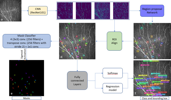
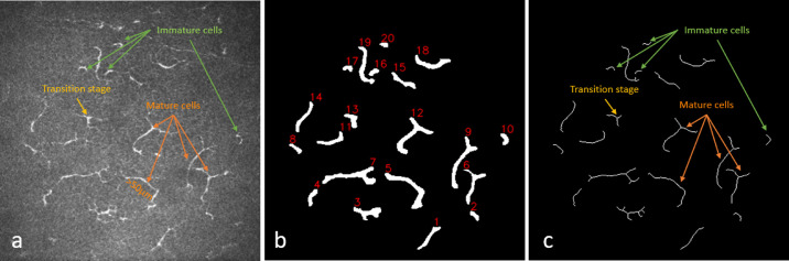
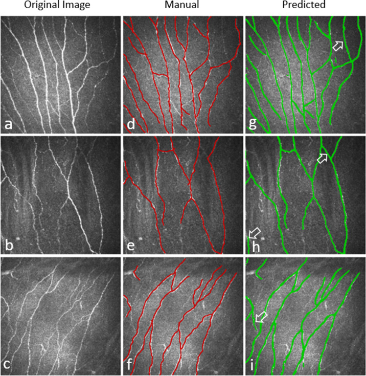
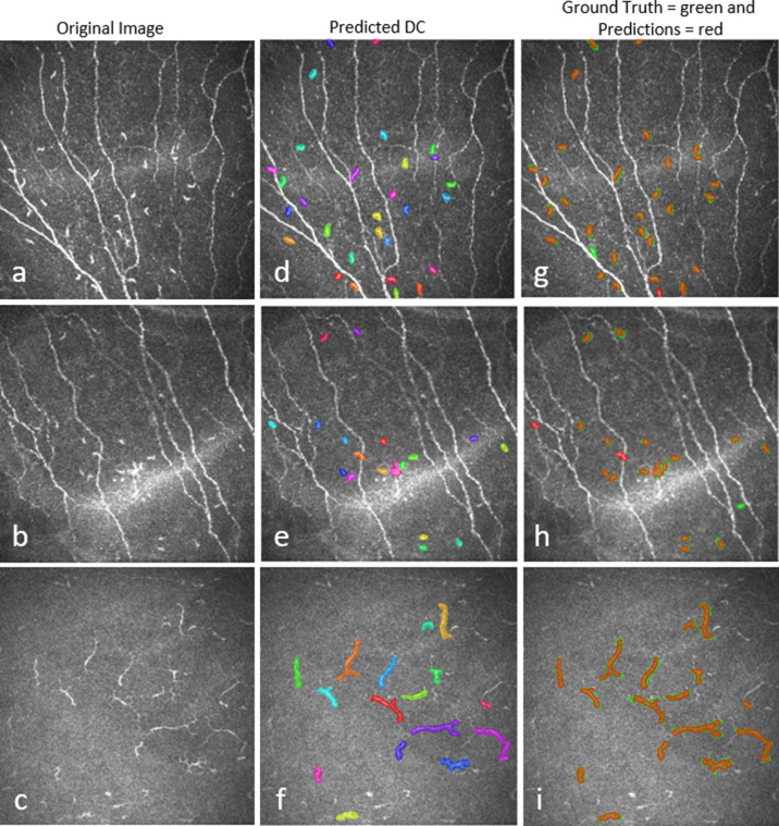
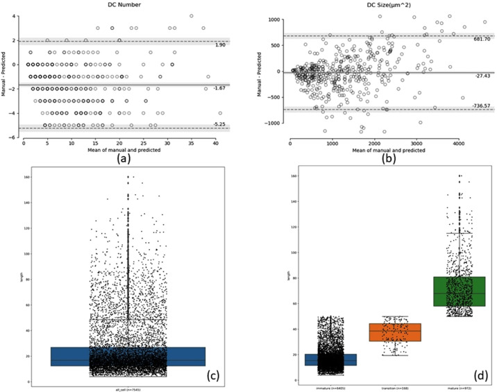
Methods: CNF and DC segmentation models were developed based on U-Net and Mask R-CNN architectures, respectively; 10-fold cross-validation was used to evaluate both models. The CNF model was trained and tested using 1097 and 122 images, and the DC model was trained and tested using 679 and 75 images, respectively, at each fold. The CNF morphology, number of nerves, number of branching points, nerve length, and tortuosity were analyzed; for DCs, number, size, and immature-mature cells were analyzed. Python-based software was written for model training, testing, and automatic morphometric parameters evaluation.

Results: The CNF model achieved on average 86.1% sensitivity and 90.1% specificity, and the DC model achieved on average 89.37% precision, 94.43% recall, and 91.83% F1 score. The interclass correlation coefficient (ICC) between manual annotation and automatic segmentation were 0.85, 0.87, 0.95, and 0.88 for CNF number, length, branching points, and tortuosity, respectively, and the ICC for DC number and size were 0.95 and 0.92, respectively.

Conclusions: Our proposed methods demonstrated reliable consistency between manual annotation and automatic segmentation of CNF and DC with rapid speed. The results showed that these approaches have the potential to be implemented into clinical practice in IVCM images.

Translational relevance: The deep learning-based automatic segmentation and quantification algorithm significantly increases the efficiency of evaluating IVCM images, thereby supporting and potentially improving the diagnosis and treatment of ocular surface disease associated with corneal nerves and dendritic cells.

Figure 1.

Detailed U-Net architecture. Each dark blue rectangular block represents a multi-channel feature map passing through 3 × 3 convolution followed by rectified linear unit (ReLU) operations. Dark gray and light blue blocks denote dropout with a rate of 0.2 and batch normalization. Orange and dark yellow blocks denote 2 × 2 max pooling and 3 × 3 transpose convolution, respectively. Green blocks denote the concatenation of feature maps. The light gray block denotes a 1 × 1 convolution operation followed by sigmoid activation. The number of convolution filters is indicated at the top of each column.

Figure 2.

Mask R-CNN architecture. The pretrained ResNet101 (light yellow box) generates feature maps (b) from the input image (a). From the feature maps, the RPN (purple box; 3 × 3 convolution with 512 filters, padding the same) generates multiple ROIs (dotted bounding box) with the help of predefined bounding boxes referred to as anchors (c). The green box denotes the ROI Align network, which takes both the proposed bounding boxes from the RPN network and the feature maps as inputs and uses this information to find the best-fitting bounding box (d) for each proposed DC. These aligned box maps are fed into fully connected layers (7 × 7 convolution with 1024 filters + 1 × 1 convolution with 1024 filters), denoted by the gray box, and then generates a class and bounding box for each object using softmax and a regression model, respectively (f). Finally, the aligned box maps are fed into the Mask classifier (4 3 × 3 convolution with 256 filters + transpose convolution with 256 filters and stride = 2 + 1 × 1 convolution + sigmoid activation), denoted by the light blue box, to generate binary masks for each object (e).

Figure 3.

Calculation of number of corneal nerves. First, the corneal nerves were divided into clusters (A, B, and C) and then each start and end point was provided with a cluster point number (A1, A2, …, B1, B2, …, C1, C2, …). After that, an abstract graph was created for each cluster using the associated nodes and edges. Then, all possible paths (if branch nerves exist in a cluster such as clusters A and C) within the abstract graph were created, and the tortuosity was calculated for each path. The main nerve was selected with the lowest tortuosity for all clusters (a). All nodes creating this main nerve were removed and the process was run again to find another main nerve if one exists (cluster C); otherwise, the remaining nerve was considered the branch nerve (cluster A) (b). If there was no additional main nerve, then the remaining nodes and edges were considered branch nerves (orange and green in cluster C) (c). Finally, the total number of corneal nerves was calculated by summing the red and orange nerves while discarding the branch nerves (green) with length less than 20% (80 µm) of the image.

Figure 4.

Immature and mature cell number calculation. (a) Original image, (b) binary segmented image with individual cell identification number, and (c) skeletonize image. The green arrows indicate immature cells (<50 µm) without dendrites, yellow arrows indicate transition-stage cells (<50 µm) with dendrites, and orange arrows indicate mature cells (>50 µm) with or without dendrites.

Figure 5.

Three examples of CNF segmentation. (a–c) Original image, (d–f) manually segmented CNFs, and (g–i) predicted CNFs by the deep learning model. White marked arrows in the predicted images indicate the thin CNFs that were predicted by the deep learning model but were not annotated in the ground-truth images.

Figure 6.

Example of an automatic CNF quantification from the segmented binary image of the deep learning model. (a) Original image, and (b) binary segmented image with automatic quantification.

Figure 7.

Bland–Altman plots present the consistency of CNF number, CNF length (mm), number of branching points, and tortuosity between manual annotation and deep learning segmentation methods. The middle solid line indicates the mean value of the two methods, and the two dotted lines indicate the limits of agreement (±1.96 SD). The gray bands indicate a confidence interval of 95%.

Figure 8.

Three examples of DC prediction by the deep learning model. (a–c) Original image, d–f) predicted DC regions, and (g–i) overlay of manual annotation and predicted DCs.

Figure 9.

DC segmentation and quantification. (a) Original image, (b) segmentation overlay with quantification parameters, and (c) skeletonized binary segmented image with cell identification numbers. The immature cell identification numbers are 2, 4, 8, 10, 16, 17, and 20; the transition-stage cell identification number is 13; and the mature cell identification numbers are 1, 3, 5, 6, 7, 9, 11, 12, 14, 15, 18, 19.

Figure 10.

Bland–Altman plots indicate the consistency of the total DC number (a) and size (µm²) (b) between manual annotation and automatic segmentation. The middle solid line indicates the mean value of the two methods, and the two dotted lines indicate the limits of agreement (±1.96 SD). The gray bands indicate a confidence interval of 95%. (c) Scatterbox plot of all segmented cells from the test images, and (d) scatterbox plot of the number of immature, transition-stage, and mature cells identified in the test images.

References

1. Craig JP, Nelson JD, Azar DT, et al. .. TFOS DEWS II Report Executive Summary. Ocul Surf. 2017; 15(4): 802–812. - PubMed
1. Stapleton F, Alves M, Bunya VY, et al. .. TFOS DEWS II Epidemiology Report. Ocul Surf. 2017; 15(3): 334–365. - PubMed
1. Craig JP, Nichols KK, Akpek EK, et al. .. TFOS DEWS II Definition and Classification Report. Ocul Surf. 2017; 15(3): 276–283. - PubMed
1. McDonald M, Patel DA, Keith MS, Snedecor SJ.. Economic and humanistic burden of dry eye disease in Europe, North America, and Asia: a systematic literature review. Ocul Surf. 2016; 14(2): 144–167. - PubMed
1. Uchino M, Schaumberg DA.. Dry eye disease: impact on quality of life and vision. Curr Ophthalmol Rep. 2013; 1(2): 51–57. - PMC - PubMed
Publication types