Learning representations of chromatin contacts using a recurrent neural network identifies genomic drivers of conformation

Abstract

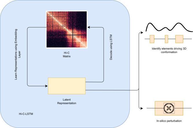
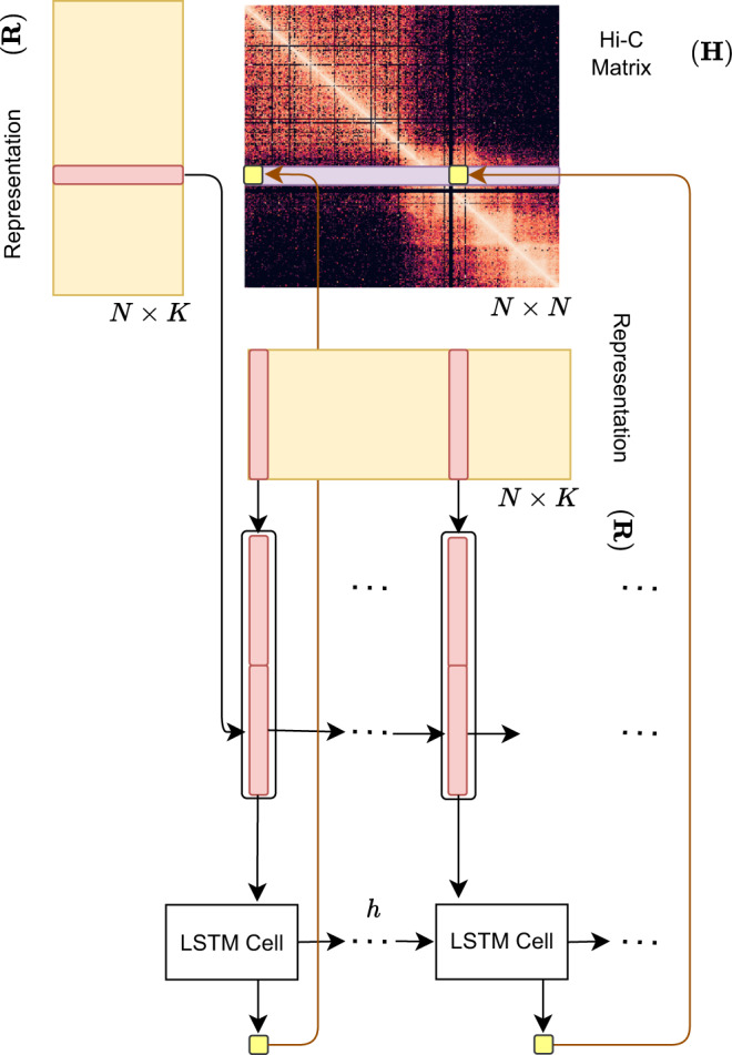
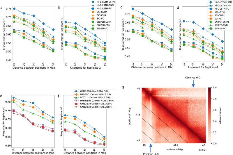
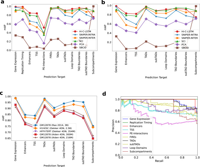
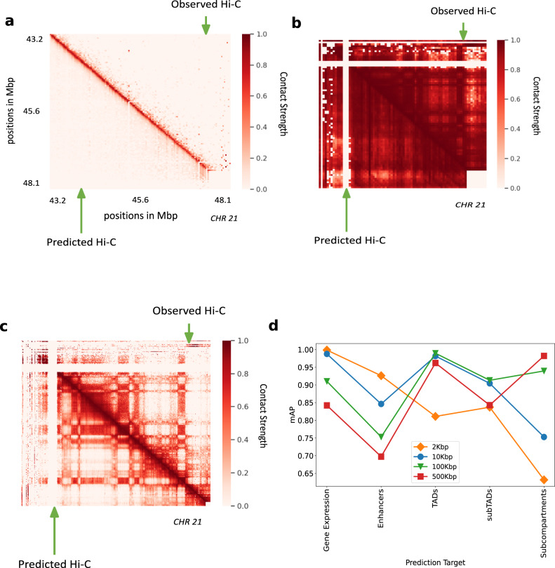
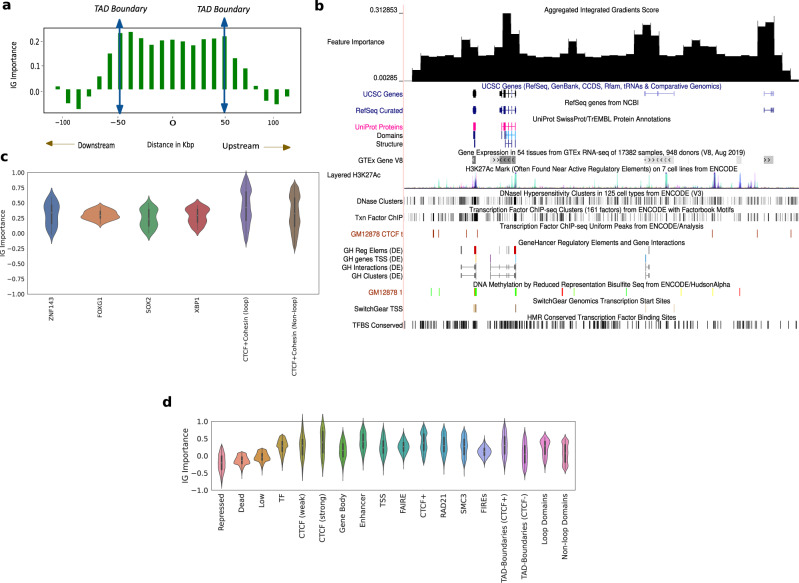
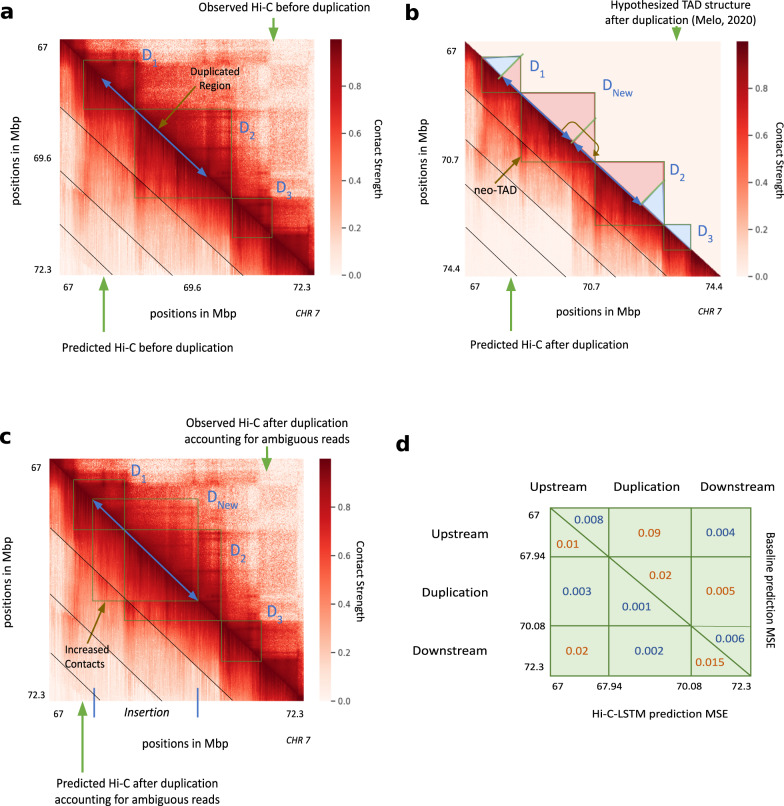
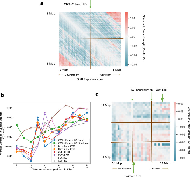
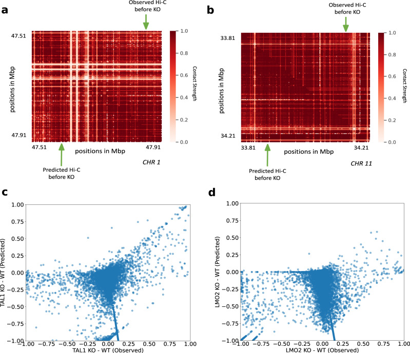
Despite the availability of chromatin conformation capture experiments, discerning the relationship between the 1D genome and 3D conformation remains a challenge, which limits our understanding of their affect on gene expression and disease. We propose Hi-C-LSTM, a method that produces low-dimensional latent representations that summarize intra-chromosomal Hi-C contacts via a recurrent long short-term memory neural network model. We find that these representations contain all the information needed to recreate the observed Hi-C matrix with high accuracy, outperforming existing methods. These representations enable the identification of a variety of conformation-defining genomic elements, including nuclear compartments and conformation-related transcription factors. They furthermore enable in-silico perturbation experiments that measure the influence of cis-regulatory elements on conformation.

Fig. 1. Overview of approach.

Hi-C-LSTM learns a K-length vector representation of each genomic position that summarizes its chromatin contacts, using an LSTM embedding neural network. The representations and LSTM decoder are jointly optimized to maximize the accuracy with which the decoder can reproduce the observed Hi-C matrix given just the representations. The resulting representations identify sequence elements driving 3D conformation through integrated gradients (IG) analysis, and they enable a researcher to perform in-silico perturbation experiments by editing the representations and observing the effect on predicted contacts.

Fig. 2. Overview of the Hi-C-LSTM model.

A trained Hi-C-LSTM model consists of a K-length representation R_i for each genomic position i and LSTM connection weights (see the “Methods” section). To predict the contact vector of a position i with all other positions, the LSTM iterates across the positions j ∈ {1…N}. For each (i, j) pair, the LSTM takes as input the concatenated representation vector (R_i R_j) and outputs the predicted Hi-C contact probability H_i,j. The LSTM hidden state h is carried over from (i, j) to (i, j + 1). This process is repeated for all N rows of the contact map by reinitializing the LSTM states. The LSTM and the representation matrix are jointly trained to minimize the reconstruction error.

Fig. 3. Accuracy with which representations reproduce the observed Hi-C matrix.

a, b The Hi-C R-squared computed using the combinations of representations from different methods and selected decoders for replicate 1 and 2 (GM12878). The horizontal axis represents the distance between positions in Mbp. The vertical axis shows the reconstruction accuracy for the predicted Hi-C data, measured by average R-squared. The R-squared was computed on a test set of chromosomes using selected decoders with the representations trained all chromosomes as input. The legend shows the different combinations of methods and decoders, read as [representation]-[decoder]. c, d Same as (a, b), but for H1-hESC. e, f Hi-C R-squared computed for different cell types. g A selected portion of the observed Hi-C map (upper-triangle) and the predicted Hi-C map (lower-triangle) in GM12878. The portion is selected from chromosome 21, between 40 and 43 Mbp. Diagonal black lines denote Hi-C-LSTM's frame boundaries (see the “Methods” section).

Fig. 4. Genomic phenomena and chromatin regions are classified using the Hi-C-LSTM representations as input.

a Prediction accuracy for gene expression, replication timing, enhancers, transcription start sites (TSSs), promoter–enhancer interactions (PEIs), frequently interacting regions (FIREs), loop and non-loop domains, and subcompartments in GM12878. The y-axis shows the mean average precision (mAP), the x-ticks refer to the prediction targets, and the legend shows the different methods compared with. b Same as (a), but for targets in H1-hESC. c mAP using Hi-C-LSTM for targets compared across cell types. d The Precision-Recall curves of Hi-C-LSTM for the various prediction targets in GM12878. The y-axis shows the Precision, the x-axis shows the Recall, and the legend shows the prediction targets.

Fig. 5. Hi-C-LSTM applied at different resolutions.

a Hi-C-LSTM predictions at 2 kbp resolution. A selected portion of the observed Hi-C map (upper-triangle) and the predicted Hi-C map (lower-triangle) in GM12878. The portion is selected from chromosome 21, between 43.2 and 48.1 Mbp. b Hi-C-LSTM predictions at 500Kbp resolution. The observed Hi-C map (upper-triangle) and the predicted Hi-C map (lower-triangle) in GM12878 for chromosome 21. c Hi-C-LSTM predictions at 100 kbp resolution. The observed Hi-C map (upper-triangle) and the predicted Hi-C map (lower-triangle) in GM12878 for chromosome 21. d The classification performance (as measured in mAP) with gene expression, enhancers, TADs, subTADs, and subcompartments of models trained at different resolutions.

Fig. 6. Hi-C-LSTM representations identify genomic elements involved in conformation through integrated gradients (IG) feature importance analysis.

a The IG feature importance averaged across different TADs of varying sizes. The vertical axis indicates the average IG importance at each position and the horizontal axis refers to relative distance between positions in kbp, upstream/downstream of the TADs. b The IG feature importance for a selected genomic locus (chr21 28–29.2 Mbp) along with genes, regulatory elements, GC percentage, CTCF signal, and conserved TFBS among others in the UCSC genome browser. We see that the feature importance scores peak at known regulatory elements, higher GC percentage, and CTCF peaks. c Violin plots of aggregated feature attribution scores for top ranked transcription factor binding sites (TFBS). The x-axis shows the labels/elements and the y-axis displays the z normalized feature importance scores from Integrated Gradients. Both at loop and non-loop regions, the scores shown are aggregated only at shared sites. d Violin plots of aggregated feature attribution scores for selected elements. The x-axis shows the labels/elements and the y-axis displays the z normalized feature importance scores from Integrated Gradients. The scores for CTCF and Cohesin subunits are aggregated genome wide. In c, d, Violin plots present summary statistics where the white dot is the median, thick gray bar is the inter-quartile range, and thin gray line is the rest of the distribution. Kernel density estimation is shown on either side of the line. Sample size for the genomic elements are calculated genome wide by considering all observations of elements according to element specific data.

Fig. 7. In-silico duplication of a 2.1 Mbp region on Chromosome 17.

In all subplots, upper and lower triangles denote observed and predicted Hi-C contact probabilities respectively, and diagonal black lines denote Hi-C-LSTM frame boundaries. a Observed and predicted Hi-C before duplication. D₁, D₂ and D₃ indicate the three pre-duplication topological domains. b Predicted Hi-C after duplication on a simulated reference genome that includes both copies. Lower triangle indicates Hi-C-LSTM predicted contacts. The true Hi-C contact matrix on this reference genome is not observable because the read mapper cannot disambiguate between the two copies. The upper triangle depicts the post-duplication topological domain structure hypothesized by Melo et al, which includes a novel topological domain D_New. c Observed and predicted Hi-C on the observed pre-duplication reference genome. Upper triangle shows observed post-duplication Hi-C data assayed by Melo et al. Lower triangle shows Hi-C-LSTM predictions, mapped to the pre-duplication reference by summing the contacts for the two copies (see the section “Results”). d Average mean-squared error (MSE) in predicting the observed data by (lower triangle) Hi-C-LSTM, and (upper triangle) a simple baseline (see the section “Results”) at the upstream, duplicated, and downstream regions.

Fig. 8. In-silico deletion of transcription factor binding sites (TFBS), orientation replacement of CTCF binding sites and TAD boundaries with and without CTCF.

a The average difference in predicted Hi-C contact strength between CTCF + Cohesin knockout (KO) and no knockout in a 2 Mb window. We simulate deletion by shifting the downstream representations upward. b Average difference in contact strength of the inferred Hi-C matrix between knockout and no knockout (y-axis) for varying distance between positions in Mbp (x-axis). The knockout experiments include TFBS knockout and convergent/divergent CTCF replacements (legend). c The genome-wide average difference in predicted Hi-C contact strength between TAD boundaries knockout and no knockout with CTCF (upper-triangle) and without CTCF (lower-triangle).

Fig. 9. In-silico anchor deletions at the TAL1 and LMO2 loci.

a, c TAL1 anchor deletion on chromosome 1. a Observed Hi-C contacts before deletion (upper-triangle), and predicted Hi-C contacts before deletion (lower-triangle). c Scatter plot of differences in contacts after and before TAL1 deletion. The x-axis shows observed differences, and the y-axis shows predicted differences. b, d LMO2 anchor deletion on chromosome 11. b Observed Hi-C contacts before deletion (upper-triangle), and predicted Hi-C contacts before deletion (lower-triangle). d Scatter plot of differences in contacts after and before LMO2 deletion. The x-axis shows observed differences, and the y-axis shows predicted differences, KO knockout, WT wild-type.

References

1. Van Berkum NL, et al. Hi-C: a method to study the three-dimensional architecture of genomes. J. Vis. Exp. 2010;39:e1869. - PMC - PubMed
1. Bengio Y, Courville A, Vincent P. Representation learning: A review and new perspectives. IEEE Trans. Pattern Anal. Mach. Intell. 2013;35:1798–828. - PubMed
1. Seide, F., Li, G. & Yu, D. Conversational speech transcription using context-dependent deep neural networks. In Proc. 12th Annual Conference of theInternational Speech Communication Association. 430–440 (2011).
1. Boulanger-Lewandowski, N., Bengio, Y. & Vincent, P. Modeling temporal dependencies in high-dimensional sequences: application to polyphonic music generation and transcription. Preprint at arXiv:1206.6392 (2012).
1. Krizhevsky A, Sutskever I, Hinton GE. Imagenet classification with deep convolutional neural networks. Commun. ACM. 2017;60:84–90.
Publication types