Interplay between traveling wave propagation and amplification at the apex of the mouse cochlea

Abstract

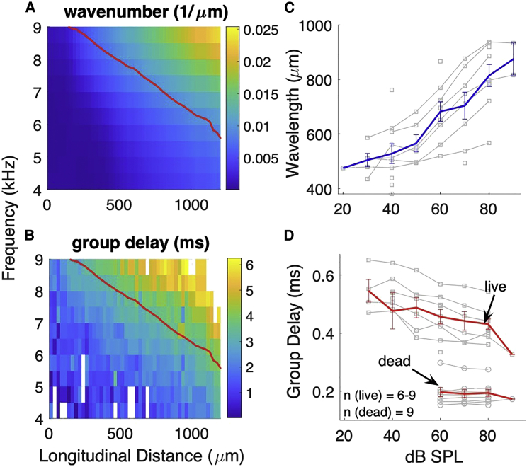
Sounds entering the mammalian ear produce waves that travel from the base to the apex of the cochlea. An electromechanical active process amplifies traveling wave motions and enables sound processing over a broad range of frequencies and intensities. The cochlear amplifier requires combining the global traveling wave with the local cellular processes that change along the length of the cochlea given the gradual changes in hair cell and supporting cell anatomy and physiology. Thus, we measured basilar membrane (BM) traveling waves in vivo along the apical turn of the mouse cochlea using volumetric optical coherence tomography and vibrometry. We found that there was a gradual reduction in key features of the active process toward the apex. For example, the gain decreased from 23 to 19 dB and tuning sharpness decreased from 2.5 to 1.4. Furthermore, we measured the frequency and intensity dependence of traveling wave properties. The phase velocity was larger than the group velocity, and both quantities gradually decrease from the base to the apex denoting a strong dispersion characteristic near the helicotrema. Moreover, we found that the spatial wavelength along the BM was highly level dependent in vivo, such that increasing the sound intensity from 30 to 90 dB sound pressure level increased the wavelength from 504 to 874 μm, a factor of 1.73. We hypothesize that this wavelength variation with sound intensity gives rise to an increase of the fluid-loaded mass on the BM and tunes its local resonance frequency. Together, these data demonstrate a strong interplay between the traveling wave propagation and amplification along the length of the cochlea.

Figure 1

Vibration measurements of the mouse cochlea using VOCTV. (A) cross-sectional OCT image of the mouse organ of Corti; RM, Reissner’s membrane; TM, tectorial membrane; OHC, outer hair cells; BM, basilar membrane. (B) BM vibration magnitude (first row), sensitivity (second row), and phase (third row) at a single longitudinal location (8.5 kHz best place) for a range of frequencies and stimulation levels (10–80 dB SPL). The postmortem response is shown in gray (60–80 dB SPL). (C) Schematic of the cochlear spiral shape illustrating the locations of our measurements, which was about half of the apical turn. (D and F) BM responses at three representative longitudinal locations for 40, 60, and 80 dB SPL stimuli. The best frequencies of 40 dB SPL are 5.5 kHz (D), 8 kHz (E), and 10.5 kHz (F) as denoted by dashed lines. (G and H) families of frequency tuning curves measured at sequential longitudinal locations along the BM for a representative live (G) and dead (H) mouse at 80 dB SPL sound. The displacement amplitudes are normalized to the peak values and phases are relative to the sound pressure inside the ear canal. (I) The place-frequency map for a live (40, 60, and 80 dB SPL) mouse. Locations are expressed as the fraction of the distance along the basilar membrane from stapes (using a tonotopic map by Müller et al. (31), with BM length L = 5.1 mm). The solid red line demonstrates the neural place-frequency map for a CBA/CAJ mouse (31). All data in this figure are from one representative mouse. To see this figure in color, go online.

Figure 2

Traveling wave properties. (A and B) BM wavenumber and group delay patterns plotted as a function of longitudinal location and stimulation frequency. Sound level was 60 dB SPL and red curves denote the best frequency versus best place (redrawn from Fig. 4, B and E). Both wavenumber and group delay increase from base to apex as well as by increasing stimulation frequency. (C and D) Wavelength (C) and group delay (D) of the 9 kHz traveling wave at the 9 kHz location plotted as a function of the stimulus level. Data from each individual mouse is plotted (gray curves) together with the averaged data (blue in C and red in D). Square and circle markers in (D) denote live and dead data, respectively. Error bars are the mean ± SE. To see this figure in color, go online.

Figure 3

Modeling the effect of a variable fluid-loaded mass on best frequency. (A) Cross section of the cochlear duct of a representative mouse. The duct dimensions were measured to be L₁ = 475 μm and L₂ = 215 μm and b = 220 μm at the 9 kHz location. (B) Level dependence of the best frequency (BF). The BF decreases monotonically with increasing sound intensity in both direct in vivo measurements (red) and estimations using added mass calculation (black and blue). The nonlinear SHO estimation ($B{F}_{nl}$ relation, blue curve) works better than linear SHO estimation ($B{F}_{lin}$ relation, black curve). The fluid added mass $\left(M_f\right)$ for both models is calculated from Eq. 14 b of (34), using geometries shown in (A). The constant $\alpha$ in the nonlinear SHO is fitted for each individual animal (with the average value of $\alpha =$ 1.05 ± 1.03 ${\left(\text{mm s}\right)}^{-2}$), using the least-squares method. Error bars show the mean ± SE (n = 10). To see this figure in color, go online.

Figure 4

Cochlear tonotopicity (A–F), BM displacement magnitude (A–C), and phase (D–F) as a function of excitation frequency (y axis) and longitudinal location (x axis) for 40 dB SPL (A and D), 60 dB SPL (B and E), and 80 dB SPL (C and F) stimuli. Values for the amplitude are normalized with respect to the frequency tuning curve at each location. The red solid curves in each panel indicate the best frequency versus best place. (G) BM gain variation with frequency and longitudinal location. The pseudocolor map represents the sensitivity difference between 40 and 80 dB SPL ($G_{40}^{80}$) responses at all measured locations (x axis) and frequencies (y axis). Solid black line denotes the best frequency of 40 dB SPL versus location. (H) Gain ($G_{40}^{80}$) at the 40 dB SPL best place (i.e., along the solid line denoted in G) as a function of the best frequency (n = 7–10). I, $Q_{10dB}$ of mechanical frequency tuning curves for the 60 dB SPL response (n = 7–10) as function of the best frequency. Error bars are the mean ± SE. To see this figure in color, go online.

Figure 5

Traveling wave profiles. Longitudinal pattern of the BM response to tones at 7 kHz (first column), 8 kHz (second column), and 9 kHz (third column); displacement magnitude (A–C), sensitivity (D–F), phase (G–I), and instantaneous waveforms (J–L) for 40, 60, and 80 dB SPL stimuli from one representative mouse. To see this figure in color, go online

Figure 6

Cochlear dispersion. (A) BM wavelength for 9 kHz sound and 30–90 dB SPL intensities versus longitudinal location. (B) BM dispersion diagram (frequency versus wavenumber) for different sound intensities at the 9 kHz best place of 40 dB SPL. (C) BM phase velocity and group velocity as a function of the longitudinal location. The color key for different sound levels is presented in (B). (D) Group velocity and phase velocity for 9 kHz, 60 dB SPL stimulation against best frequency of different longitudinal locations along the cochlea. Error bars are the mean ± SE. To see this figure in color, go online.

Figure 7

Testing for scaling symmetry. Spatial profiles of displacement magnitude (A–C) and phase (D–F) for three different stimulus levels (40, 60, and 80 dB SPL) from one representative mouse. The stimulus frequencies were 6 kHz (A and D), 7 kHz (B and E), and 9 kHz (C and F). The thin black curves are the actual in vivo measurements from multiple points. The thick gray curves represent scaling symmetry extrapolations based on single-point measurements, made at the sites of the red vertical lines. (G and H) Tuning curve magnitudes (G) and phases (H) for 46 different longitudinal locations along the BM. Stimulation is 60 dB SPL for (G–L) and frequencies in the x axes are normalized to the BF of each tuning curve. (I and J) The coefficient of variation (CV) of the normalized tuning curves. (K and L) Averaged CV (n = 5) for displacement (K) and phase (L) against normalized frequency. Error bars are the mean ± SE. To see this figure in color, go online.

References

-
- V Bekesy G. McGraw Hill; New York: 1960. Experiments in Hearing.
- Zwislocki J. Review of recent mathematical theories of cochlear dynamics. J. Acoust. Soc. Am. 1953;25:743–751. doi: 10.1121/1.1907170. - DOI
- Helmholtz H.L.F. Cambridge University Press; 1912. On the Sensations of Tone as a Physiological Basis for the Theory of Music.
Publication types
MeSH terms
Grants and funding
LinkOut - more resources
Full Text Sources
Miscellaneous