Estimating the localization spread function of static single-molecule localization microscopy images

Abstract

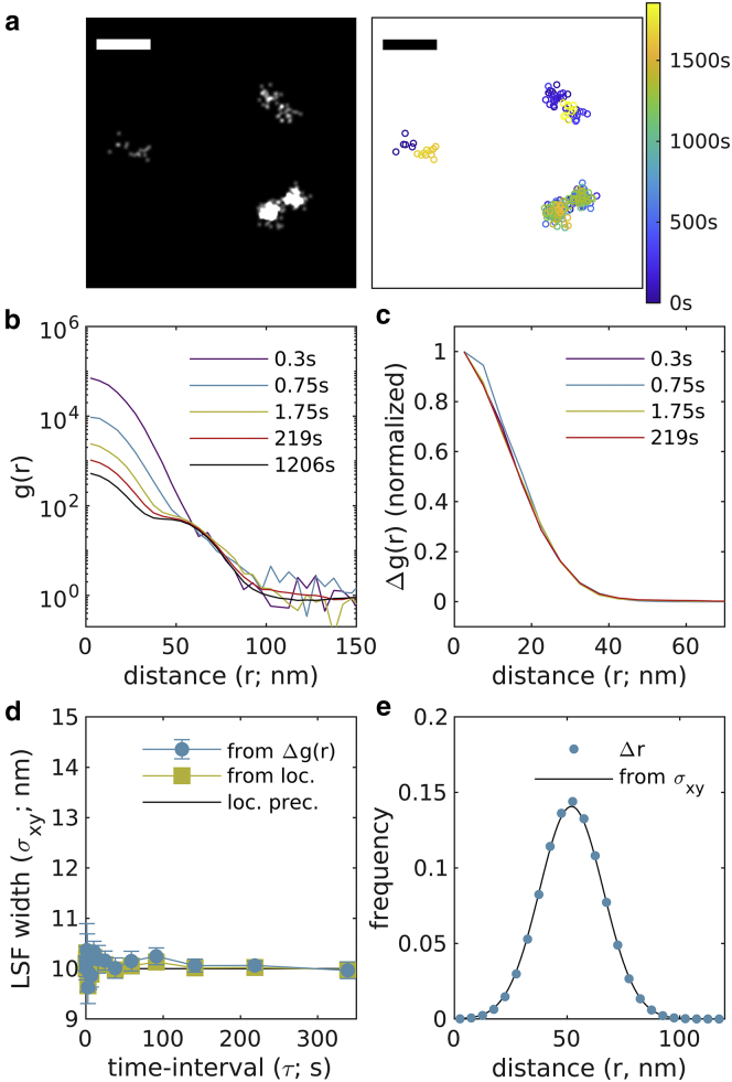
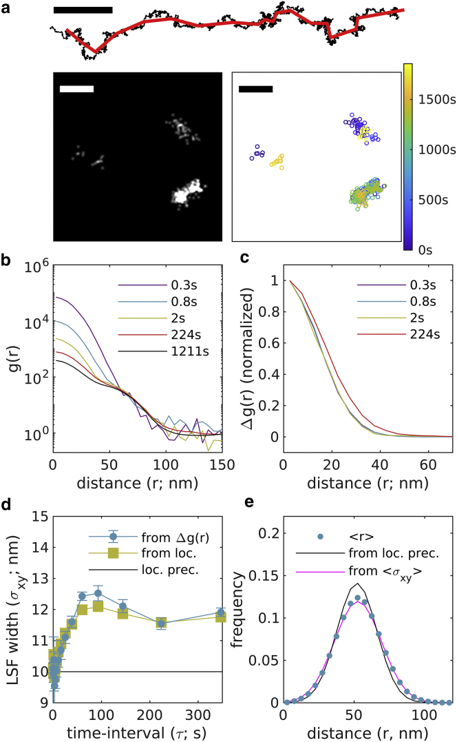
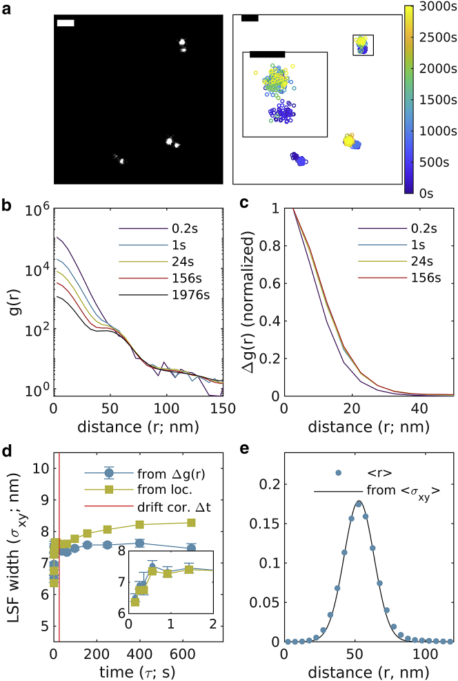
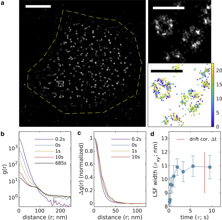
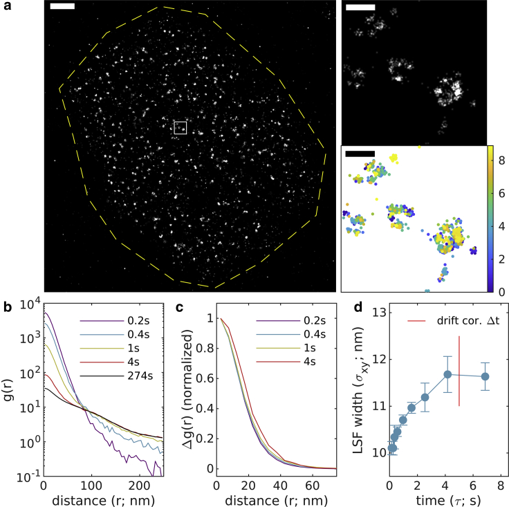
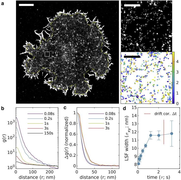
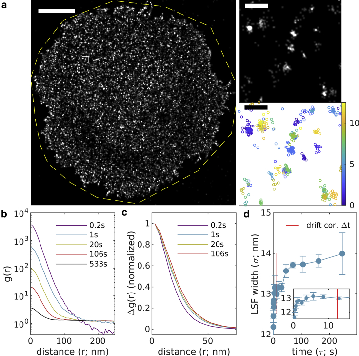
Single-molecule localization microscopy (SMLM) permits the visualization of cellular structures an order of magnitude smaller than the diffraction limit of visible light, and an accurate, objective evaluation of the resolution of an SMLM data set is an essential aspect of the image processing and analysis pipeline. Here, we present a simple method to estimate the localization spread function (LSF) of a static SMLM data set directly from acquired localizations, exploiting the correlated dynamics of individual emitters and properties of the pair autocorrelation function evaluated in both time and space. The method is demonstrated on simulated localizations, DNA origami rulers, and cellular structures labeled by dye-conjugated antibodies, DNA-PAINT, or fluorescent fusion proteins. We show that experimentally obtained images have LSFs that are broader than expected from the localization precision alone, due to additional uncertainty accrued when localizing molecules imaged over time.

Figure 1

Validation of approach through simulation. (a) Simulations consist of randomly positioned pairs of molecules positioned 50 nm apart in random orientations. Reconstructed image (left; 1 nm pixels, 3 nm Gaussian blur) and scatterplot of localizations with color representing the observation time (right) for a small subset of the simulated plane. Scale bar, 100 nm. A reconstructed image showing a larger field of view is shown in Fig. S4. (b) Autocorrelations as a function of displacement $g(r,\tau )$, tabulated from simulations for time interval windows centered at the values shown. (c) $\text{Δ}g\left(r,\tau \right)=g\left(r,\tau \right)-g\left(r,{\tau }_{\max }=1206s\right)$ for the examples shown in (b). (d) $\text{Δ}g\left(r,\tau \right)$ are fit to $\text{Δ}g\left(r,\tau \right)\propto \exp \left\{-r^2/4{\sigma }_{xy}^2\right\}$ to extract the width of the LSF in each lateral dimension, which in this case is the same as the LSF width deduced by grouping localizations with their associated molecules (from loc.) and the simulated localization precision (loc. prec.) at all time intervals. Error bars represent estimates of the standard error obtained through bootstrapping. (e) The distribution of displacements between different molecules on the same ruler are well described by a model incorporating the localization precision (10 nm) and the separation distance (50 nm). To see this figure in color, go online.

Figure 2

Validation of approach through simulation with drift and drift correction. (a) The simulation from Fig. 1 with applied drift (black) and drift correction (red) as shown in the trajectory above. Reconstructed image (left; 1 nm pixels, 3 nm Gaussian blur) and scatterplot of localizations with color representing the observation time (right) for a small subset of the simulated plane. Scale bar, 100 nm. (b) Autocorrelations as a function of displacement $g(r,\tau )$, tabulated from simulations for time interval windows centered at the values shown. (c) $\text{Δ}g\left(r,\tau \right)=g\left(r,\tau \right)-g\left(r,{\tau }_{\max }=1211s\right)$ for the examples shown in (b). (d) $\Delta g(r,\tau )$ are fit to $\text{Δ}g\left(r,\tau \right)\propto \exp \left\{-r^2/4{\sigma }_{xy}^2\right\}$ to extract the width of the effective LSF in each lateral dimension. In this case, the LSF width varies with time interval, closely following the LSF width measured by grouping localizations with molecules (from loc.). Error bars represent estimates of the standard error obtained through bootstrapping. (e) The distribution of displacements between different molecules on the same ruler are well described by a model incorporating the average LSF width ($⟨{\sigma }_{xy}⟩=11.8\text{nm}$) and the known separation distance (50 nm). To see this figure in color, go online.

Figure 3

Experimental observations of DNA origami rulers labeled with AlexaFluor647. (a) Reconstructed image (left; 1 nm pixels, 3 nm Gaussian blur) and scatterplot of localizations with color representing the observation time (right) for a small subset of the observed plane. Scale bars, 100 nm and 50 nm (inset). A larger field of view from this image is shown in Figure S6. (b) Autocorrelations as a function of displacement $g(r,\tau )$, tabulated from localizations for time interval windows centered at the values shown. (c) $\text{Δ}g\left(r,\tau \right)=g\left(r,\tau \right)-g\left(r,{\tau }_{\max }=1976s\right)$ for the examples shown in (b). (d) $\text{Δ}g\left(r,\tau \right)$ are fit to $\text{Δ}g\left(r,\tau \right)\propto \exp \left\{-r^2/4{\sigma }_{xy}^2\right\}$ to extract the width of the LSF in each lateral dimension which varies with time interval, closely following the LSF width measured by grouping localizations with DBSCAN segmented molecules (from loc.). Error bars represent estimates of the standard error obtained through bootstrapping. The resulting average LSF width for this image is $⟨{\sigma }_{xy}⟩=$ 7.48 ± 0.07 nm. (e) The distribution of displacements between pairs of fluorophores on the same ruler. Fitting to a Gaussian shape with width given by the measured $⟨{\sigma }_{xy}⟩$ produces $⟨r⟩=$ 52.2 ± 0.2 nm. To see this figure in color, go online.

Figure 4

Experimental observations of DNA origami rulers imaged with DNA PAINT, using an Atto655 imaging strand. (a) Reconstructed image (left; 1 nm pixels, 3 nm Gaussian blur) and scatterplot of localizations with color representing the observation time (right) for a small subset of the observed plane. Scale bar, 100 nm. A larger field of view from this image is shown in Figure S7. (b) Autocorrelations as a function of displacement $g(r,\tau )$, tabulated from localizations for time interval windows centered at the values shown. (c) $\text{Δ}g\left(r,\tau \right)=g\left(r,\tau \right)-g\left(r,{\tau }_{\max }=609s\right)$ for the examples shown in (b). (d) $\text{Δ}g\left(r,\tau \right)$ are fit to $\text{Δ}g\left(r,\tau \right)\propto \exp \left\{-r^2/4{\sigma }_{xy}^2\right\}$ to extract the width of the LSF in each lateral dimension, which varies with time interval, closely following the LSF width measured by grouping localizations with DBSCAN segmented molecules (from loc.). Error bars represent estimates of the standard error obtained through bootstrapping. The resulting average LSF width for this image is$⟨{\sigma }_{xy}⟩=$ 8.8 ± 0.2 nm. (e) The distribution of displacements between different molecules on the same ruler. Fitting to a Gaussian shape with width given by the measured $⟨{\sigma }_{xy}⟩$ produces $⟨r⟩=$ 82.5 ± 0.3 nm. To see this figure in color, go online.

Figure 5

Experimental observations of nuclear pore complexes within primary mouse neurons, antibody-labeled with AlexaFluor647. (a) (Left) Reconstructed image (10 nm pixels, 10 nm Gaussian blur) with yellow dashed line indicating the region of interest interrogated. (Right) A magnified subset from the white square region of larger image (1 nm pixels, 4 nm Gaussian blur) along with a scatterplot of localizations with color representing the observation time. Scale bars, 2 μm (left) and 200 nm (right top and bottom). (b) Autocorrelations as a function of displacement $g(r,\tau )$, tabulated from localizations for time interval windows centered at the values shown. (c) $\text{Δ}g\left(r,\tau \right)=g\left(r,\tau \right)-g\left(r,{\tau }_{\max }=685s\right)$ for the examples shown in (b). (d) $\Delta g(r,\tau )$ are fit to $\text{Δ}g\left(r,\tau \right)\propto \exp \left\{-r^2/4{\sigma }_{xy}^2\right\}$ to extract the LSF width in each lateral dimension. Error bars represent estimates of the standard error obtained through bootstrapping. The average LSF width for this image is $⟨{\sigma }_{xy}⟩=$ 10.9 ± 0.8 nm. To see this figure in color, go online.

Figure 6

Experimental observations of clathrin-coated pits within CH27 B cells, imaged using a nanobody-coupled Atto655 DNA-PAINT scheme. (a) (Left) Reconstructed image (16 nm pixels, 20 nm Gaussian blur) with yellow dashed line indicating the region of interest interrogated. (Right) A magnified subset from the white square region of larger image (1 nm pixels, 4 nm Gaussian blur) along with a scatterplot of localizations with color representing the observation time. Scale bars, 2 μm (left) and 200 nm (right top and bottom). (b) Autocorrelations as a function of displacement $g(r,\tau )$, tabulated from localizations for time interval windows centered at the values shown. (c) $\text{Δ}g\left(r,\tau \right)=g\left(r,\tau \right)-g\left(r,{\tau }_{\max }=274s\right)$ for the examples shown in (b). (d) $\Delta g(r,\tau )$ are fit to $\text{Δ}g\left(r,\tau \right)\propto \exp \left\{-r^2/4{\sigma }_{xy}^2\right\}$ to extract the LSF width in each lateral dimension. Error bars represent estimates of the standard error obtained through bootstrapping. The average resolution for this image is $⟨{\sigma }_{xy}⟩=$ 11.6 ± 0.3 nm. To see this figure in color, go online.

Figure 7

Experimental observations of F-actin on the ventral surface of a CH27 B cell using phalloidin-AlexaFluor647. (a) (Left) Reconstructed image (50 nm pixels, 50 nm Gaussian blur) with yellow dashed line indicating the region of interest interrogated. (Right) A magnified subset from the white square region of larger image (1 nm pixels, 10 nm Gaussian blur) along with a scatterplot of localizations with color representing the observation time. Scale bars, 5 μm (left) and 500 nm (right top and bottom). (b) Autocorrelations as a function of displacement $g(r,\tau )$, tabulated from localizations for time interval windows centered at the values shown. (c) $\text{Δ}g\left(r,\tau \right)=g\left(r,\tau \right)-g\left(r,{\tau }_{\max }=150s\right)$ for the examples shown in (b). (d) $\text{Δ}g\left(r,\tau \right)$ are fit to $\text{Δ}g\left(r,\tau \right)\propto \exp \left\{-r^2/4{\sigma }_{xy}^2\right\}$ to extract the LSF width in each lateral dimension. The timescale of the drift correction is shown in red. Error bars represent estimates of the standard error obtained through bootstrapping. The average resolution for this image is $⟨{\sigma }_{xy}⟩=$ 11.8 ± 1.5 nm. To see this figure in color, go online.

Figure 8

Experimental observations of membrane anchor peptide Src15-mEos3.2 on the ventral surface of a CH27 B cell. (a) (Left) Reconstructed image (50 nm pixels, 50 nm Gaussian blur) with yellow dashed line indicating the region of interest interrogated. (Right) A magnified subset from the white square region of larger image (1 nm pixels, 6 nm Gaussian blur) along with a scatterplot of localizations with color representing the observation time. Scale bars, 5 μm (left) and 200 nm (right top and bottom). (b) Autocorrelations as a function of displacement $g(r,\tau )$, tabulated from localizations for time interval windows centered at the values shown. (c) $\text{Δ}g\left(r,\tau \right)=g\left(r,\tau \right)-g\left(r,{\tau }_{\max }=533s\right)$ for the examples shown in (b). (d) $\text{Δ}g\left(r,\tau \right)$ are fit to $\text{Δ}g\left(r,\tau \right)\propto \exp \left\{-r^2/4{\sigma }_{xy}^2\right\}$ to extract the LSF width in each lateral dimension. The timescale of the drift correction is shown in red. Error bars represent estimates of the standard error obtained through bootstrapping. The average resolution for this image is $⟨{\sigma }_{xy}⟩=$ 13.7 ± 0.2 nm. To see this figure in color, go online.

References

1. Rust M.J., Bates M., Zhuang X. Sub-diffraction-limit imaging by stochastic optical reconstruction microscopy (STORM) Nat. Methods. 2006;3:793–795. doi: 10.1038/nmeth929. - DOI - PMC - PubMed
1. Heilemann M., Margeat E., et al. Tinnefeld P. Carbocyanine dyes as efficient reversible single-molecule optical switch. J. Am. Chem. Soc. 2005;127:3801–3806. doi: 10.1021/ja044686x. - DOI - PubMed
1. Hess S.T., Girirajan T.P.K., Mason M.D. Ultra-high resolution imaging by fluorescence photoactivation localization microscopy. Biophys. J. 2006;91:4258–4272. doi: 10.1529/biophysj.106.901116. - DOI - PMC - PubMed
1. Betzig E., Patterson G.H., et al. Hess H.F. Imaging intracellular fluorescent proteins at nanometer resolution. Science. 2006;313:1642–1645. doi: 10.1126/science.1127344. - DOI - PubMed
1. Sharonov A., Hochstrasser R.M. Wide-field subdiffraction imaging by accumulated binding of diffusing probes. Proc. Natl. Acad. Sci. USA. 2006;103:18911–18916. doi: 10.1073/pnas.0609643104. - DOI - PMC - PubMed
Publication types
MeSH terms
LinkOut - more resources