Advances in human intracranial electroencephalography research, guidelines and good practices

Abstract

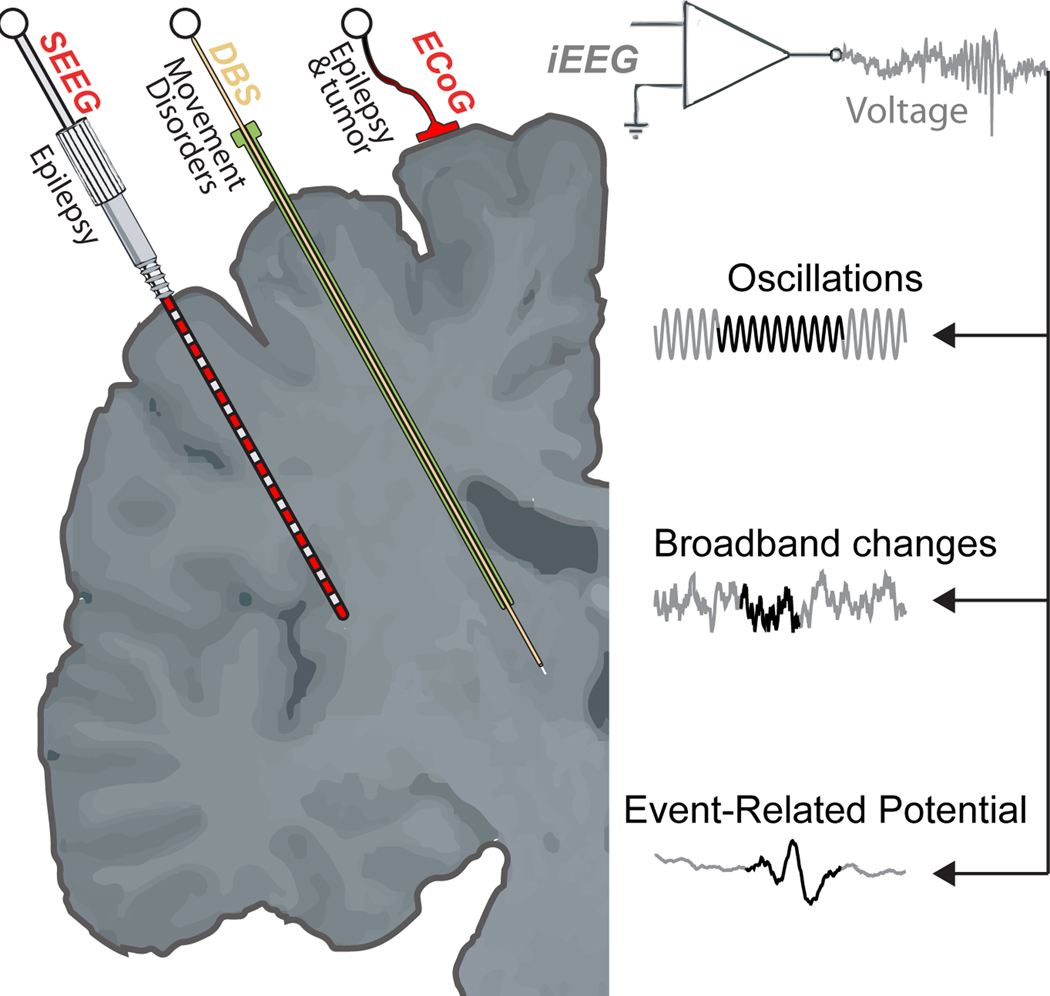
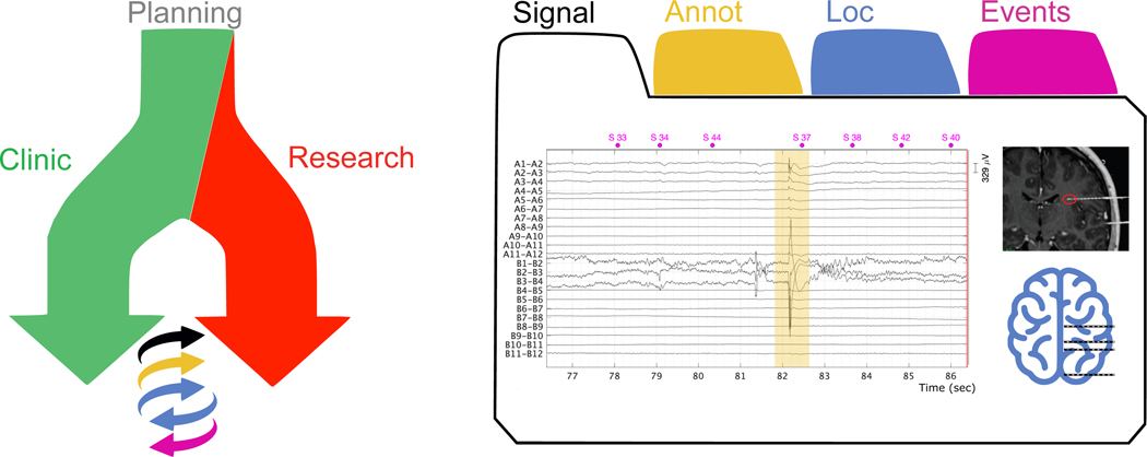
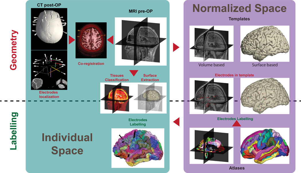
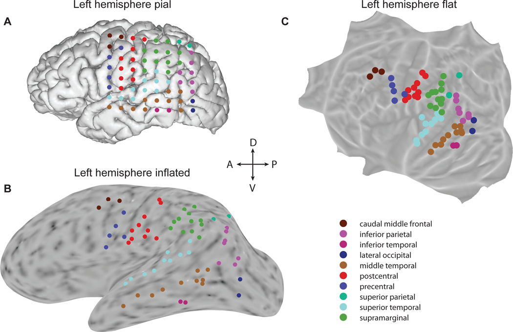
Since the second-half of the twentieth century, intracranial electroencephalography (iEEG), including both electrocorticography (ECoG) and stereo-electroencephalography (sEEG), has provided an intimate view into the human brain. At the interface between fundamental research and the clinic, iEEG provides both high temporal resolution and high spatial specificity but comes with constraints, such as the individual's tailored sparsity of electrode sampling. Over the years, researchers in neuroscience developed their practices to make the most of the iEEG approach. Here we offer a critical review of iEEG research practices in a didactic framework for newcomers, as well addressing issues encountered by proficient researchers. The scope is threefold: (i) review common practices in iEEG research, (ii) suggest potential guidelines for working with iEEG data and answer frequently asked questions based on the most widespread practices, and (iii) based on current neurophysiological knowledge and methodologies, pave the way to good practice standards in iEEG research. The organization of this paper follows the steps of iEEG data processing. The first section contextualizes iEEG data collection. The second section focuses on localization of intracranial electrodes. The third section highlights the main pre-processing steps. The fourth section presents iEEG signal analysis methods. The fifth section discusses statistical approaches. The sixth section draws some unique perspectives on iEEG research. Finally, to ensure a consistent nomenclature throughout the manuscript and to align with other guidelines, e.g., Brain Imaging Data Structure (BIDS) and the OHBM Committee on Best Practices in Data Analysis and Sharing (COBIDAS), we provide a glossary to disambiguate terms related to iEEG research.

Keywords: ECoG; Electrocorticogram; Good research practice; Intracranial recording in humans; Stereotactic electroencephalography; sEEG.

Figure 1

Intracranial EEG recordings and basic signal features. iEEG can be measured using three different recording strategies: stereotactic EEG (sEEG), Electrocorticogram (ECoG), and deep-brain stimulation (DBS). Signal features are generally characterized as oscillations, broadband changes, and event-related potentials.

Figure 2

Schematic representation of the interaction between clinic and research. Left panel: starting from surgical planning, with involvement over time of the clinical and research procedure. The clinical team provides the research team with the iEEG data, imaging data, and clinical annotations (e.g., epileptic activity). In return, the research team(s) can provide the precise localization of the electrodes (Loc), and activation tasks with associated event-related results regarding brain functions (Events). Right panel: illustration of the different types of data in an iEEG study: iEEG (Signal) and imaging data, clinical annotations (Annot), electrode locations (Loc) and (responses to) task-related events (Event).

Figure 3

Canonical framework of iEEG electrode localization using illustrations utilized as a sanity-check for the outputs of each step of the processing pipeline.

Figure 4

Examples of differences in signals related to the surrounding tissue. A: ECoG signal as a function of electrode location. The left panel shows the location of the ECoG grid on the individual's brain. Three electrodes are highlighted (but not at scale): over a blood vessel and sulcus (in yellow), on the bank of a gyrus and close to a blood vessel and sulcus (in orange), and over a gyrus (in red). The insert shows the angiogram (vessels) projected on the cortical surface. The right panel shows 30 sec of the high-frequency band signal (frequency analysis using Morlet wavelets, high-frequency band power extracted in 1-Hz bins and averaged over 45–120 Hz with 1-second smoothing) for the three electrodes (same amplitude scale). B: sEEG signal as a function of electrode location. The left panel shows the location of three sEEG electrodes (not at scale): one in the skull (in purple), one at the interface of the soft tissues (in pink), and one in the gray matter (in red). The right panel shows 2 sec of the raw signal for the three electrodes (same amplitude scale).

Figure 5

Brain depiction and electrode visualization ECoG electrodes are color-coded according to the anatomical label that corresponds to their location. Electrodes are shown on (A) the original pial surface of the participant’s brain, where the grid structure may be best appreciated, (B) the inflated cortical surface and (C) the flattened cortical surface (in this case based on the projection onto the fsaverage brain). The inflated and flattened surfaces are colored according to surface curvature calculated in FreeSurfer, where darker gray indicates the sulci, and lighter gray indicates gyri. The best choice of representation (pial, inflated or flat) depends on the coverage of electrodes as well as which areas are to be compared.

Figure 6

Oblique slice aligned with sEEG shaft. Graphical interface allowing the display of MRI slices aligned with a selected sEEG shaft highlighted in blue in the list. In the oblique slice sEEG contacts are represented as green dots. In the 3D view the plane corresponding with the shaft axis is depicted in green with a transparent brain, sEEG contacts are here represented as black spheres.

Figure 7

Electrode display and data interpolation. For ECoG (Panel A) and sEEG (Panel C), the amplitude of the iEEG signal is represented at their corresponding 3D locations, then projected orthogonally along the three axes (as in a glass brain view), and depicted on MRI slices. In panels B (ECoG) and D (sEEG), the amplitude of the signals is interpolated on a 3D brain (left column) and on an inflated brain (right column, with light gray indicating gyri and dark gray indicating sulci). Signal interpolation was done using a sphere of 5mm for the upper row and 15 mm for the lower row. In panel B the ECoG electrodes are indicated in green; in panel D two sEEG shafts are indicated in red and green. While activity is identical in the upper row and in the lower row, the extent of the interpolation changes the rendering.

Figure 8

Examples of artifacts due to eye and mouth movements. A. Ocular artifacts in sEEG. The EOG and iEEG were recorded while the participant was asked to either blink or move his eyes leftward (upper left panel, color-coded in blue and red respectively). EOG single-trial averaging (n=16) shows time-locked muscular-related activity on cardinal EOGs (upper middle panel); and on vertical and horizontal EOGs obtained through bipolar referencing (upper right panel). Intracranial EEG was recorded from 252 electrodes relative to a reference located in the white matter (yellow circle on the lower left panel). Broadband Event Related Potentials computed with both a monopolar reference (WMR) and a bipolar reference (Bp) are depicted for a frontal and a posterior electrode. For the frontal sEEG electrode, the artifact time-locked to muscular activity recorded with EOG is visible with the monopolar reference and is reduced when the bipolar montage reference is applied. The posterior electrode shows activity that is not reduced by the bipolar referencing and that is delayed with regards to EOG activity. The frontal electrode shows muscular activity that has passively diffused from the eye muscles, while the posterior electrode shows local neural activity that is consecutive to the eyes movement (e.g. change in visual input or corollary signal). B. Oral artifacts in sEEG. The participant was asked to clench his teeth ten times while sEEG was recorded. Broadband and high-frequency activity recorded from frontal electrodes reveal artifacts time-locked to jaw-contraction (color-coded in pink and in green respectively).

Figure 9

Interfaces examples for artifact detection A. The Power Spectrum Density (PSD) of all channels can help to identify artifacted channels with artifacts (in red). B. A display per channel and per trial can be used to identify short-lived artifacts. The heatmap represents for every trial (along the horizontal axis) and every channel (along the vertical axis) a metric (here the variance) which is color-coded from blue to yellow. The panels to the right and below the heatmap represent the maximum variance over trials and over channels, respectively. A channel with high variance over most trials is highlighted by the magenta rectangle. A trial with high variance over channels is highlighted by the orange rectangle.

Figure 10

Interface showing reference switch. Illustration of displays with two different montages (unipolar reference on the left and bipolar reference on the right). The montages are selected graphically in a dedicated menu (here in Brainstorm). When switching from the unipolar to the bipolar montage, the low- and high-frequency artifacts shared over all channels are reduced.

Figure 11

Signal-to-noise ratio (SNR) as a function of the number of trials. Activity was recorded in the primary auditory cortex of a participant while listening to pure tones (1000 Hz). A. Activity is depicted for different numbers of averaged trials. The broadband ERP is depicted on the left, the magnitude envelope of high-frequency activity is shown on the right. B. SNR varies with the number of trials used for averaging. SNR was computed using the maximum amplitude of the activity divided by the variance over the baseline (S/N).

Figure 12

Influence of the reference montage on iEEG signal analysis. A. Location of sEEG electrodes in the brain of the participant (axial slice on the left, coronal slice on the right). B. ERP computed with different reference montages, respectively in black for monopolar white matter reference (WMR), dark blue for common average reference (CAR), light blue for local average reference (LAR, using all electrodes of the sEEG shaft), and red for bipolar reference (Bp). A schematic of the sEEG shaft is depicted to illustrate the spatial organization of the activity and especially the phase reversal revealed by the bipolar montage (e.g., at the level of channel #11). C. Power from time-frequency analysis computed with different reference montages, respectively from left to right: WMR, CAR, LAR and Bp. Both CAR and LAR introduce a strong correlation of high-frequency activity over channels, absent in the WMR. D. Phase Concentration Index from time-frequency analysis computed with different reference montages, respectively from left to right: Bp, WMR, CAR and LAR. Both CAR and LAR introduce a strong correlation of high-frequency activity over channels, absent in the WMR. Note the presence of induced activity, that is only visible in the power depiction (part C), and of evoked activity that is visible in both the depictions of power and Phase Concentration Index (e.g., see channel 8–9 with Bp montage). E. Phase angle distribution represented for different reference montages, respectively from left to right: Bp, WMR, CAR and LAR. The data corresponds to the red square indicated in the time-frequency plane of channel 6. While the absolute angle measure varies with the reference montage, the relative measure (i.e., PCI) is consistent across reference montages.

Figure 13

Baseline correction and time frequency representation. The same time-frequency representation of power is depicted with different baselining methods computed from −1 sec to −0.5 s. Within a frequency range (orange) and two time ranges of interest (purple and red), the mean and the mean-absolute-deviation are depicted at the bottom and on the side. The choice of the baseline method enhances/reduces the visibility of particular features in the data (for instance the 1/f effect, see sections 4.2.3.3 and 4.2.3.4.1).

Figure 14

Distinction and interaction between prediction, i.e., hypothesis based confirmatory research, and postdiction or exploratory research.

Figure 15

Combining group-level and patient-level anatomical analysis. Group-level functional activations show HFA response components at specific latencies. This allows the definition of a Region of Interest (ROI) for further investigation. Panel A shows a strong group-level (n=67) HFA response in the basal temporal cortex 400 ms after the display of a written word during a reading task contrasting attended vs. ignored words. Panel B shows a group representation of all iEEG sites in the ROI in the left temporal lobe (pink sphere), across all patients. Subsequently, each site can be visualized onto a 3D representation of the corresponding individual brain (panel C), to understand how the strength of the response depends on its precise localization relative to specific individual anatomical landmarks, such as the lingual gyrus. Repeating the same procedure for all subjects and sites within the ROI leads to a detailed anatomical characterization of iEEG sites with a homogenous functional response (visualizations and analysis were made with HiBoP).

References

1. Abel TJ, Rhone AE, Nourski KV, Granner MA, Oya H, Griffiths TD, Tranel DT, Kawasaki H, Howard MA, 2014. Mapping the temporal pole with a specialized electrode array: technique and preliminary results. Physiol. Meas 35, 323–337. 10.1088/0967-3334/35/3/323 - DOI - PMC - PubMed
1. Abramian D, Eklund A, 2019. Refacing: Reconstructing Anonymized Facial Features Using GANS, in: 2019 IEEE 16th International Symposium on Biomedical Imaging (ISBI 2019). Presented at the 2019 IEEE 16th International Symposium on Biomedical Imaging (ISBI), IEEE, Venice, Italy, pp. 1104–1108. 10.1109/ISBI.2019.8759515 - DOI
1. Adhikari A, Sigurdsson T, Topiwala MA, Gordon JA, 2010. Cross-correlation of instantaneous amplitudes of field potential oscillations: a straightforward method to estimate the directionality and lag between brain areas. J. Neurosci. Methods 191, 191–200. 10.1016/j.jneumeth.2010.06.019 - DOI - PMC - PubMed
1. Alagapan S, Lustenberger C, Hadar E, Shin HW, Frӧhlich F, 2019. Low-frequency direct cortical stimulation of left superior frontal gyrus enhances working memory performance. NeuroImage 184, 697–706. 10.1016/j.neuroimage.2018.09.064 - DOI - PMC - PubMed
1. Alday PM, 2019. How much baseline correction do we need in ERP research? Extended GLM model can replace baseline correction while lifting its limits. Psychophysiology 56, e13451. 10.1111/psyp.13451 - DOI - PubMed
Publication types