Neural network organization for courtship-song feature detection in Drosophila

Abstract

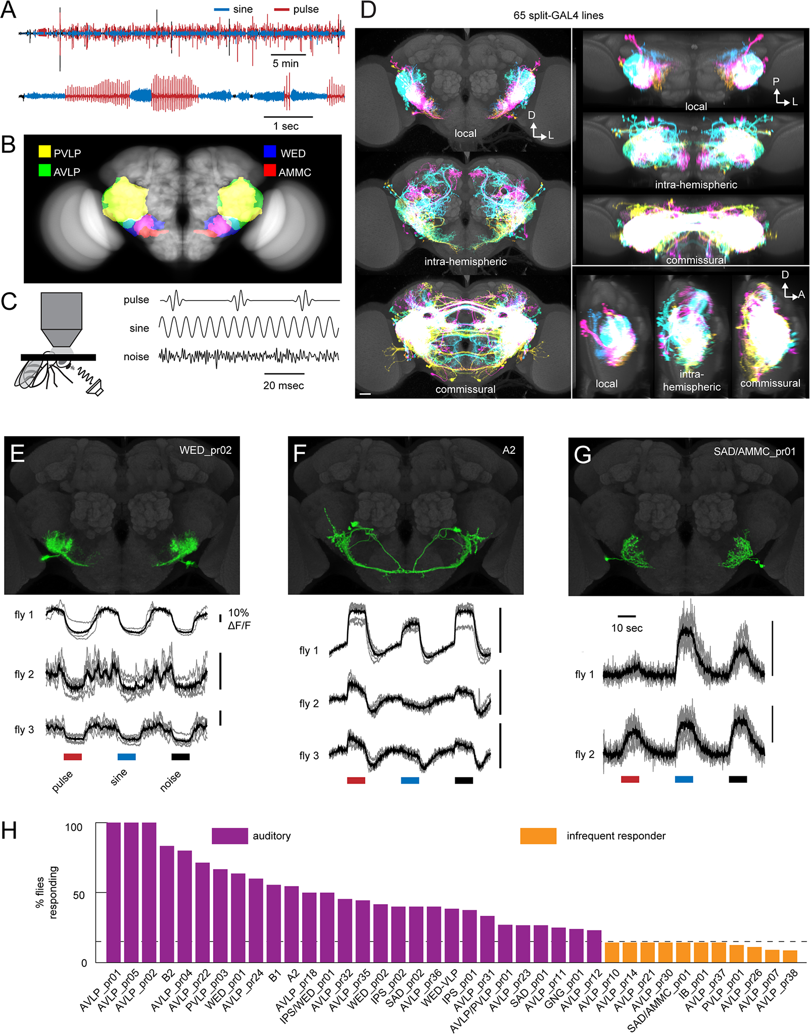
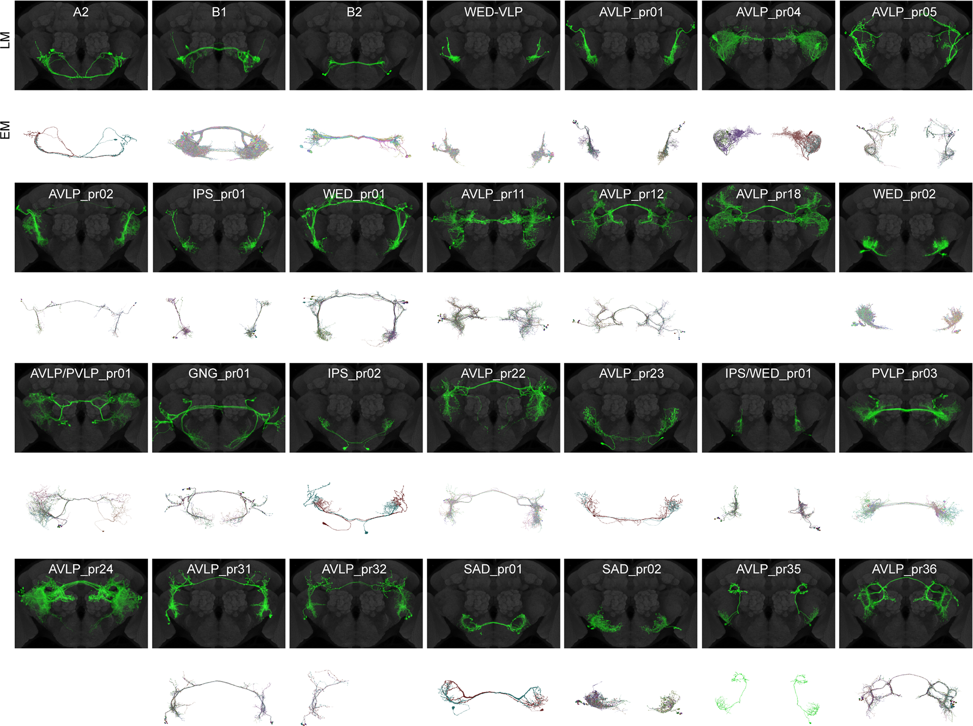
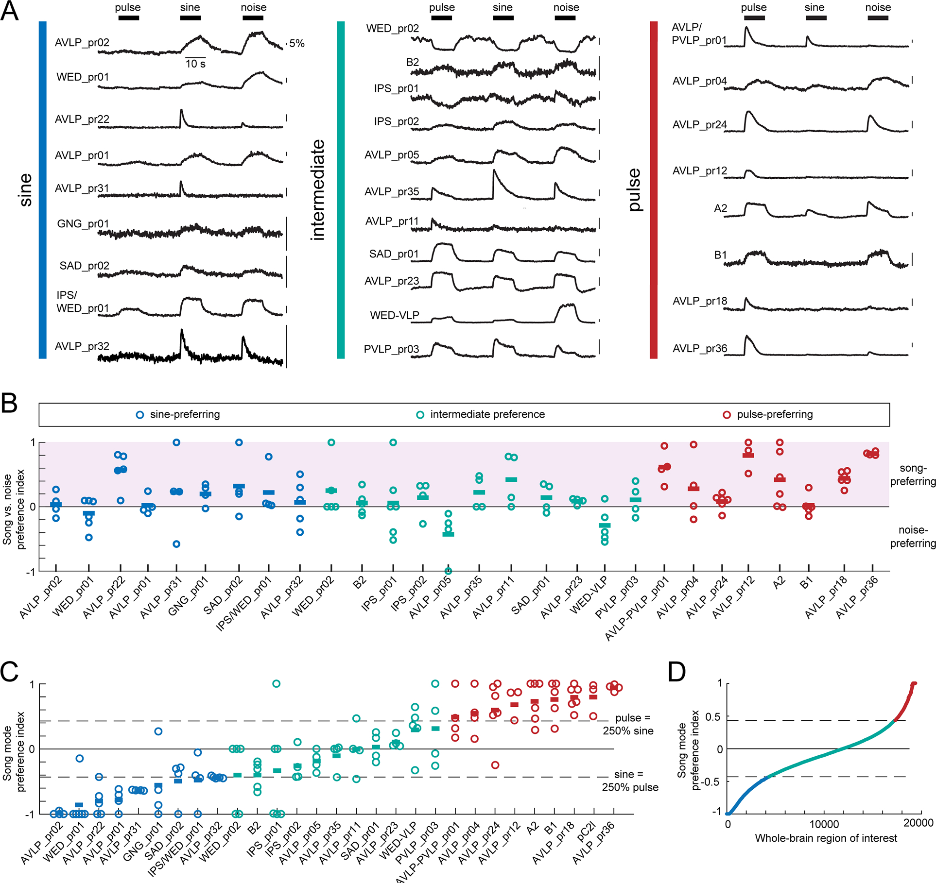
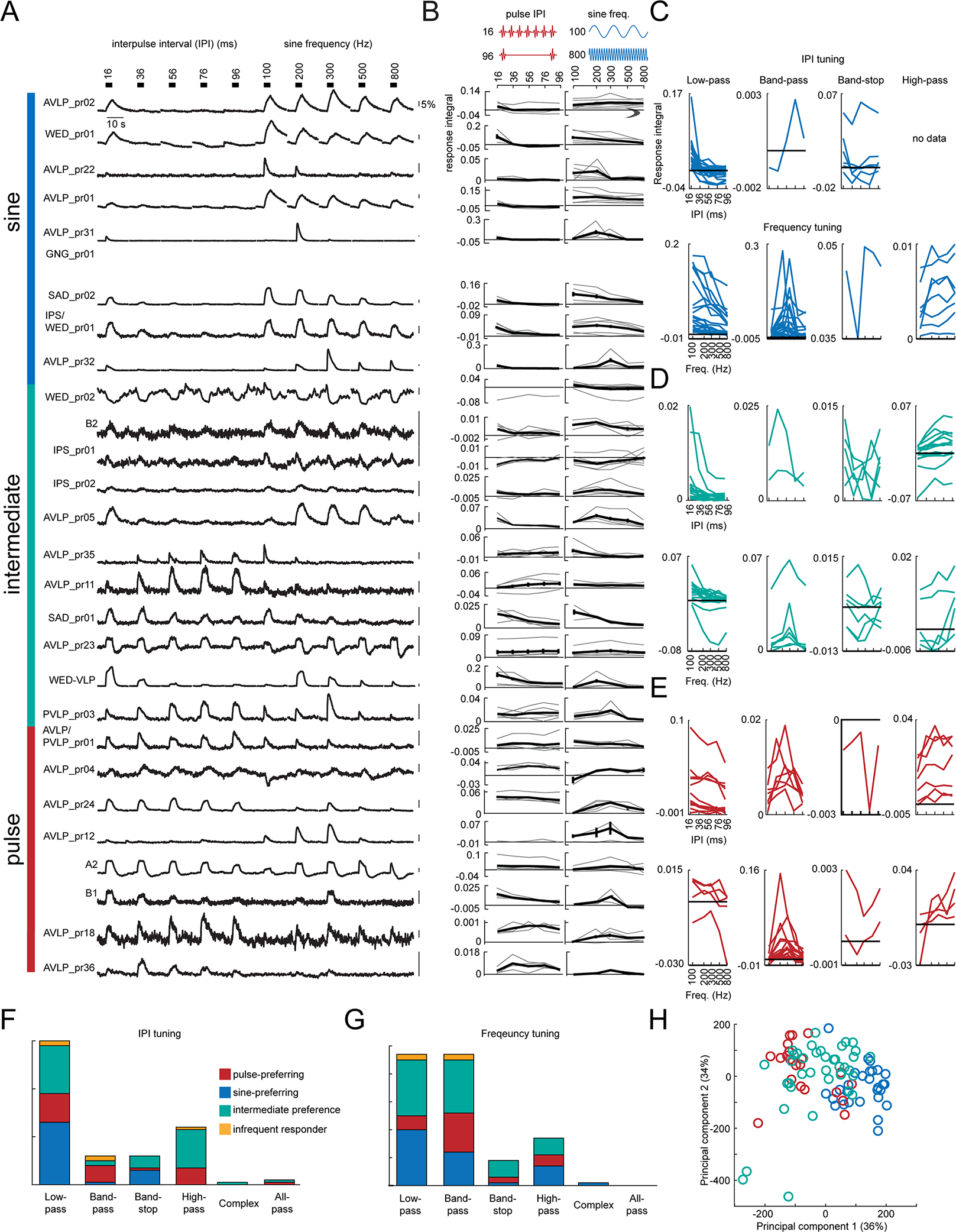
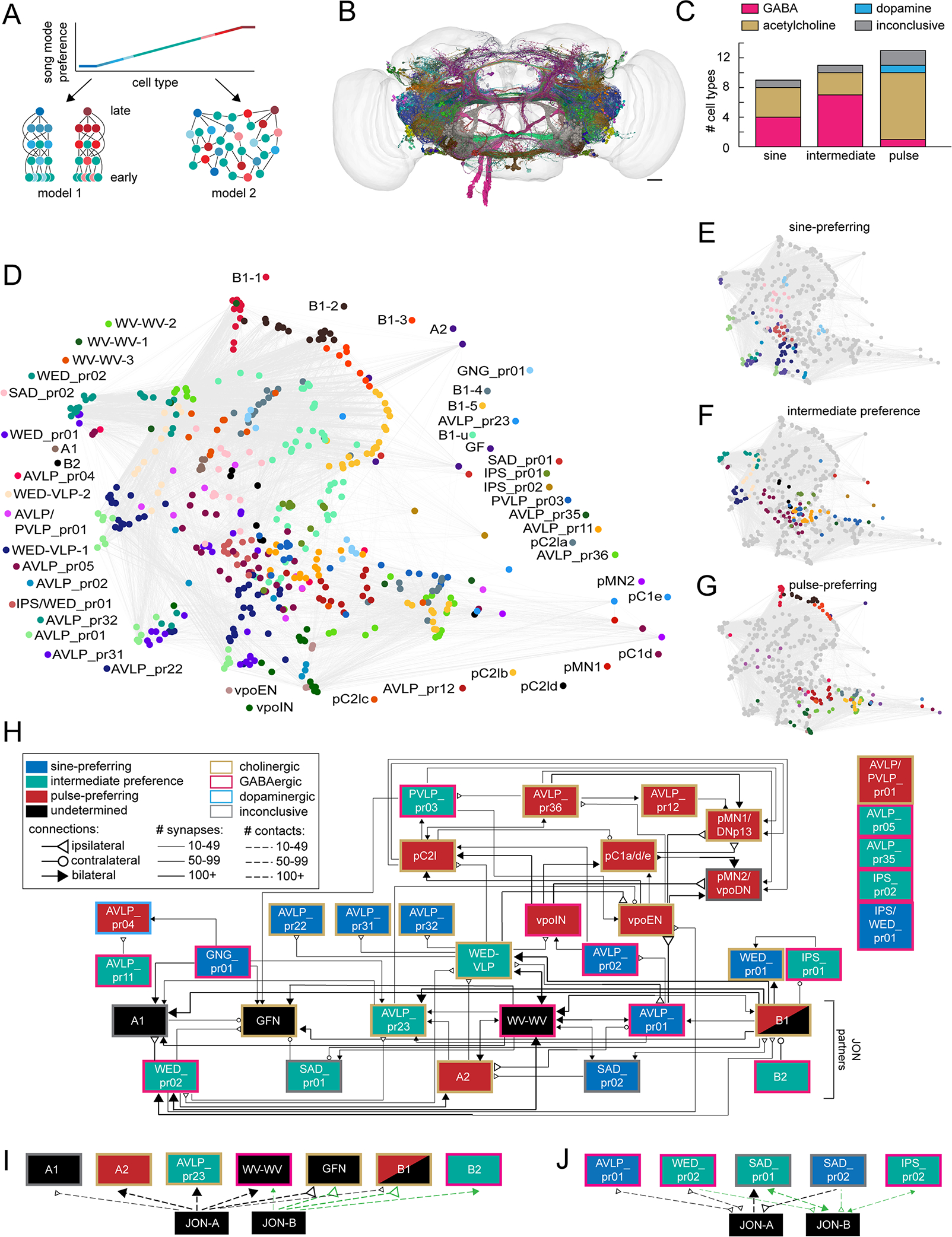
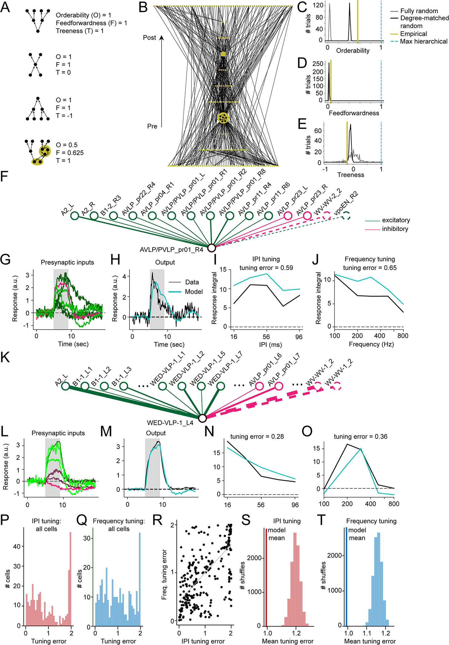
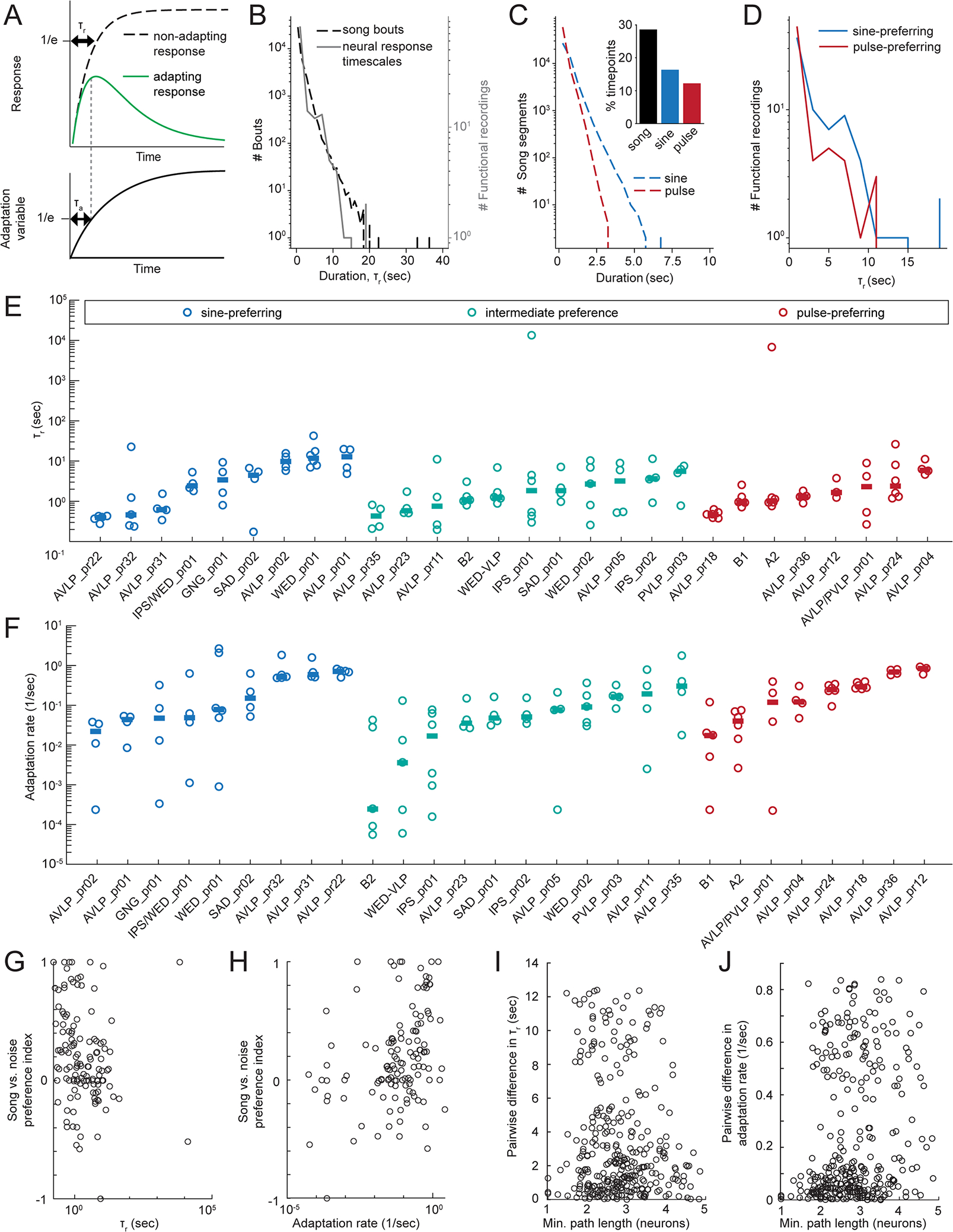
Animals communicate using sounds in a wide range of contexts, and auditory systems must encode behaviorally relevant acoustic features to drive appropriate reactions. How feature detection emerges along auditory pathways has been difficult to solve due to challenges in mapping the underlying circuits and characterizing responses to behaviorally relevant features. Here, we study auditory activity in the Drosophila melanogaster brain and investigate feature selectivity for the two main modes of fly courtship song, sinusoids and pulse trains. We identify 24 new cell types of the intermediate layers of the auditory pathway, and using a new connectomic resource, FlyWire, we map all synaptic connections between these cell types, in addition to connections to known early and higher-order auditory neurons-this represents the first circuit-level map of the auditory pathway. We additionally determine the sign (excitatory or inhibitory) of most synapses in this auditory connectome. We find that auditory neurons display a continuum of preferences for courtship song modes and that neurons with different song-mode preferences and response timescales are highly interconnected in a network that lacks hierarchical structure. Nonetheless, we find that the response properties of individual cell types within the connectome are predictable from their inputs. Our study thus provides new insights into the organization of auditory coding within the Drosophila brain.

Keywords: acoustic communication; auditory; calcium imaging; connectomics; neural network; sensory responses.

Figure 1.. Anatomic and functional screen for auditory neurons.

A) Microphone recording from a single wild-type (CS-Tully strain) male fly paired with a virgin female. The top trace shows song over 30 minutes, and the bottom trace shows a close-up of song bouts consisting of switches between the pulse and sine song modes. B) Primary auditory neurons called Johnston Organ neurons in the antenna project to the antennal mechanosensory and motor center (AMMC) in the central brain. Auditory information is then routed to downstream areas including the wedge (WED), anterior ventrolateral protocerebrum (AVLP), and posterior ventrolateral protocerebrum (PVLP). See Table S1 for neuropil abbreviations. C) Schematic showing two-photon calcium imaging set-up with sound delivered to the aristae (left) and calibrated, synthetic acoustic stimuli used to search for auditory responses (right). 100 msec of each stimulus is shown. D) Overlaid images of the split-GAL4 collection’s local interneurons, intra-hemispheric projection neurons, or commissural neurons, segmented from aligned images of the split GAL4 collection (see also Data S1A–B) and shown as maximum projections from the front (left), top (top right), and side (bottom right). Each cell type was colored randomly. D: dorsal; L: lateral; P: posterior; A: anterior. Scale bar: 25 microns. E-G) Calcium responses to pulse, sine, and noise stimuli from three cell classes (see also Figure S1D–E). In the calcium traces, each trial is shown in grey and the mean across trials is shown in black. H) Percentage of imaged flies from each cell class with auditory responses. We defined auditory cell classes as those in which >15% (dotted line) of imaged flies responded to the pulse, sine, or noise stimuli. If at least 1 fly but fewer than 15% of imaged flies responded, we termed the cell class an ‘infrequent responder’. If no flies responded (out of 4–6 total flies), we termed the cell class ‘non-auditory’. Numbers of flies imaged ranged from 4–17 for auditory cell classes, and from 7–23 for infrequently responding cell classes. See Table S2 and Data S1C for cell class images and names. See also Tables S1–2.

Figure 2.. Light microscopic (LM) and electron microscopic (EM) images of auditory WED/VLP cell types.

Aligned central brains with expression patterns of WED/VLP neuron classes digitally segmented (see Data S1B–C). Only those cell classes with auditory responses are shown. Gray: nc82. Below each brain expression pattern are the EM reconstructions (identified and proofread in FlyWire.ai, see Table S3) corresponding to each cell class. There was insufficient information in the split-GAL4 and stochastic labeling expression patterns to resolve the EM reconstructions representing two cell classes (AVLP_pr18 and AVLP_pr24). EM reconstructions representing cell type AVLP_pr32 were only found in one hemisphere. AVLP_pr01 and AVLP_pr02 share morphological similarities with vpoINs, which provide sound-evoked inhibition onto descending neurons called vpoDNs that contribute to vaginal plate opening (Wang et al., 2020b). Based on both FlyWire and hemibrain connections, vpoINs (defined as inputs to vpoDN with morphology consistent with vpoINs) consist of two subtypes: one with a commissure, and one with a medial projection that does not cross the midline. This leads us to conclude that AVLP_pr02 are likely the commissural vpoINs, but AVLP_pr01 are a cell type independent from vpoINs. See also Figures S2 and S3 and Tables S2 and S3.

Figure 3.. Auditory WED/VLP neurons show a continuum of preferences for sine and pulse song modes.

A) Trial-averaged representative calcium traces for a single fly from each cell class in response to pulse, sine, and noise stimuli. Vertical colored bars indicate the pulse- vs. sine-preference of each cell class given in (C). B) The integrals of responses to pulse, sine, and noise were used to calculate a song vs. noise preference index, which ranges from −1 (strongest noise preference) to 1 (strongest song preference) (see Methods and Figure S1A–B). The color of the dots reflect the pulse- vs. sine-preference of each cell class given in (C). Each dot represents the responses of one fly, and horizontal lines represent the mean within each cell type. To identify sine-preferring cell types, we required the mean preference index across flies to be below −0.43, which corresponds to a sine response that is at least 250% that of pulse. To identify pulse-preferring cell types, we required the mean preference index across flies to be above −0.43, which corresponds to a pulse response that is at least 250% that of sine. All other cell types were classified as having intermediate song mode preference. The song mode preference index for pC2l was calculated using data from a previous study . Each dot represents the responses of one fly, and horizontal lines represent the mean within each cell type. There was no correlation between song vs. noise preference in (B) and song mode preference in (C) (Spearman’s rho=0.15, p=0.071, n=143 flies). Tan dots indicate cell types that contact JONs (see Figure S4B). See also Figure S1D–F for response variability and Figure S2 for the neuropils innervated by neurons from each song mode preference class. D) The song mode preference index for 19,389 auditory-responsive regions of interest (ROIs) from the entire central brain, obtained via pan-neuronal imaging in a previous study . See also Figures S1–3 and Table S2.

Figure 4.. Pulse rate (interpulse interval) and frequency tuning.

A) Trial-averaged representative calcium traces in response to pulse rate (interpulse interval (IPI)) and sine frequency stimuli. B) Pulse rate (left) and sine frequency (right) tuning curves. The tuning curves from individual flies are shown in grey, and the average across flies is shown in black. Error bars report standard error. C-E) Tuning curves for each fly recorded in the data set. Tuning curves are colored according to the song mode preference of each WED/VLP neuron type. F-G) Histogram of IPI (F) and frequency (G) tuning types across the dataset. Responses that were roughly equal for every stimulus were classified as all-pass, and responses that did not fit any other category were classified as complex (see Methods). H) Principal components analysis (PCA) on the response integrals elicited by IPI and frequency stimuli. Each dot represents one recording, and the color represents the song mode preference for each cell type. PC1 positively correlates with responses to 100 and 200 Hz stimuli, and negatively correlates with responses to 36–96 ms IPI stimuli. PC2 positively correlates with responses to 16 and 36 ms stimuli, and negatively correlates with responses to 100 and 800 Hz stimuli. See also Table S2.

Figure 5.. The auditory connectome.

A) Two models for the organization of auditory pathways underlying the observed continuum of song mode preferences. Each circle represents a cell type, and each line represents synaptic connections. Red = pulse-preferring, blue = sine-preferring, and green = intermediate preference (see Figure 3C). The shading of red and blue neurons indicates the strength of pulse or sine preference, respectively. In model 1, neurons selective for pulse and sine are separated into distinct pathways, with neurons of intermediate preferences playing roles in both pathways (left). Within-mode connections sharpen tuning for song features. See Figure S3 for evidence of anatomic separation between pulse and sine pathways, supporting model 1. In model 2, neurons of different song mode preferences are highly interconnected at all levels without hierarchical organization (right). Downstream neurons may pool the responses of diversely tuned neurons to establish selectivity for a variety of song parameters. B) To test these models, we examined synaptic connections among auditory neurons (N=479 neurons from 48 cell types) in an electron microscopic volume of an entire female fly brain (see Figure S4A). D) Representation of the synaptic connectivity of auditory neurons using uniform manifold approximation and projection (UMAP). Each dot represents one neuron, the color of the dot represents the cell type, and lines represent synaptic connections. E-G) Same as D but for only sine-preferring (E), intermediate preference (F), or pulse-preferring (G) neurons. H) Flow-chart diagram of the auditory connectome. Each box represents a cell type, and each line represents a synaptic connection (see Methods for connection criteria). The song mode preference of A2, B2, and WED-VLP come from recordings from the split-GAL4 lines labeling those neurons (Figure 3C; Table S2), and the song preferences of several higher-order and descending neurons (pC2la-c, vpoEN, vpoIN, pC1a,d,e, pMN1/DNp13, and pMN2/vpoDN) come from previous studies ^,–. Cell types shown in black boxes have not had their sine/pulse preference determined. B1 shading reflects the observation that the split-GAL4 line we imaged from, while pulse-preferring, labels only a handful of B1 cells, and the tuning of the remaining B1 cells remains to be determined (but see . Five cell types formed no connections with other neurons in the dataset. See Figure S5 for neurotransmitter determination and connections of auditory cells with previously reported subtypes (ie, WED-VLP, WV-WV, and B1). See Methods for how the connectivity diagram was formed from identified reconstructions in FlyWire.ai. I) Diagram of connections between JONs and auditory cell types in which JONs are presynaptic (as measured by number of membrane contacts; see Methods and Figure S4B–E). Connections with JON-As are shown in black, and connections with JON-Bs are shown in orange. J) Same as (I) for connections in which auditory cell types are presynaptic to JONs. See also Figures S4–5 and Tables S2–3.

Figure 6.. Evaluating the hierarchical structure of the auditory network and emergence of postsynaptic tuning curves from connectome-weighted presynaptic responses.

A) Measures of hierarchical structure (orderability, feedforwardness, and treeness) for four simple networks (reproduced from ); each gold region highlights a strongly connected component (a set of neurons all mutually reachable from one another via at least one directed path). B) Hierarchically displayed node-weighted graph condensation of the empirically measured auditory network. Each node in the condensation is a strongly connected component of the original auditory network, with node size indicating the number of neurons in the component (minimum 1 neuron, maximum 124 neurons). Connections are oriented upward with postsynaptic targets displayed above presynaptic sources. C) Orderability of the auditory network, computed from the original network and the graph condensation (A), as compared to 300 instantiations (trials) of either a fully random network (with only neuron count and connection probability matched to the original auditory network) or degree-matched random network (in which each neuron’s incoming and outgoing connection numbers were inherited from the empirical network but connections were otherwise randomized). D) Feedforwardness of the auditory network, as compared to fully random and degree-matched random networks. The low value arises from most paths passing through the largest connected component. E) Treeness of the auditory network, as compared to fully random and degree-matched random networks. Prior to analysis, connections between two neurons in the original network were only counted if at least 10 synapses were detected (171 out of 476 neurons were unconnected to the main network and left out of the calculations). A maximally hierarchical network has a feedforwardness, orderability, and treeness of 1 (cyan; C-E). F) Schematic of network model used to compute neural responses and tuning for cell AVLP/PVLP_pr01_R4 (lower node). Upper nodes represent input neurons and lines indicate synaptic connections. Solid lines represent inputs from imaged split-GAL4 lines and dotted lines represent inputs from neurons outside our imaging dataset. G) Normalized responses of cells presynaptic to AVLP/PVLP_pr01_R4 (15 total, 2 without tuning data), in response to 36 ms IPI stimulus. Coloring shows weight of presynaptic cell onto postsynaptic cell, with brighter green or red indicating stronger excitatory and inhibitory weights, respectively. The grey box indicates when the stimulus was on. H) Observed postsynaptic response to the same 36 ms IPI stimulus (black) vs response modeled by feeding presynaptic responses through the network model (teal). I) IPI tuning curves from observed and modeled postsynaptic responses, computed by integrating responses from stimulus onset to 4 seconds post stimulus offset. J) Same as (I) for sine frequency tuning. K-O) Same as (F-J) for cell WED-VLP-1_L4 (29 total, 3 without tuning data). Ellipses in (K) indicate additional neurons in the data that we did not have room to show in the diagram. P) Root mean squared error between true and modeled IPI tuning curves across all cells with both post- and presynaptic tuning data (N = 306 cells); tuning curves were z-scored first to compare shape rather than magnitude. Q) Same as (P) for sine frequency tuning curves. R) IPI tuning error vs. sine frequency tuning error across cells (N=306 cells, R = 0.671, p < 10^−39; Wald test with zero-slope null hypothesis). S) Histogram of mean errors computed by shuffling true relative to modeled tuning curves across cells (10000 shuffles, p < 0.0001, computed by counting number of shuffles yielding a mean value less than the observed mean). Vertical line indicates the mean from (P). T) Same as (S) for frequency tuning curves (p < 0.0001). Vertical line indicates the mean from (Q). See also Table S2.

Figure 7.. Response time courses are matched to song statistics.

A) Schematic of calculation of response time constant τ_r and adaptation time constant τ_a (see Methods). The neuron’s total response is modeled by the green curve. B) Distribution of song bout durations (dotted line) and best fit response timescales τ_r to imaged neurons (grey). Song data was recorded during a naturalistic courtship assay in a previous experiment ; data available from ). Song was recorded with a microphone then downsampled to 30 Hz; each downsampled frame was labeled either sine, pulse, or quiet. Bouts were defined as contiguous singing periods (quiet periods of only 1 frame were ignored in separating bouts). C) Distribution of contiguous pulse and sine song segment durations. Inset shows a histogram of % time with any song, pulse, or sine. D) Distribution of τ_r for pulse- vs. sine-preferring neurons. E) Response time courses for each cell type. Each dot represents the recording from one fly and horizontal lines indicate across-fly means. F) Same as E for adaptation rate (1/τ_a). G) Song vs. noise preference vs. τ_r for all recordings. We found a negative correlation between τ_r and song vs. noise preference (Spearman rank correlation, rho=−0.31, p<0.001, n=125 flies). H) Song vs. noise preference vs. adaptation rate for all recordings. We found a positive correlation between adaptation rate and song vs. noise preference (Spearman rank correlation, rho=0.35, p<0.0001, n=125 flies). I) Difference in τ_r between every pair of neurons and the corresponding path length between each pair. There was no significant correlation (Spearman rank correlation, rho=−0.049, p=0.20, n=676 pairs of neurons). J) Same as (I) for adaptation rates. There was a weak but significant correlation between similarity of adaptation rate and path length (Spearman rank correlation, rho=0.24, p<1e-9, n=676 pairs of neurons). See also Table S2.

References

1. Akre KL, Farris HE, Lea AM, Page RA, and Ryan MJ (2011). Signal perception in frogs and bats and the evolution of mating signals. Science 333, 751–752. - PMC - PubMed
1. Baker CA, Clemens J, and Murthy M (2019). Acoustic Pattern Recognition and Courtship Songs: Insights from Insects. Annu. Rev. Neurosci. 42, 129–147. - PMC - PubMed
1. Hedwig BG (2016). Sequential Filtering Processes Shape Feature Detection in Crickets: A Framework for Song Pattern Recognition. Front. Physiol. 7, 46. - PMC - PubMed
1. Nieder A, and Mooney R (2020). The neurobiology of innate, volitional and learned vocalizations in mammals and birds. Philos. Trans. R. Soc. Lond. B Biol. Sci. 375, 20190054. - PMC - PubMed
1. Behr O, and von Helversen O (2004). Bat serenades—complex courtship songs of the sac-winged bat (Saccopteryx bilineata). Behavioral Ecology and Sociobiology 56, 106–115.
Publication types
LinkOut - more resources