Hippocampal place cells have goal-oriented vector fields during navigation

Abstract

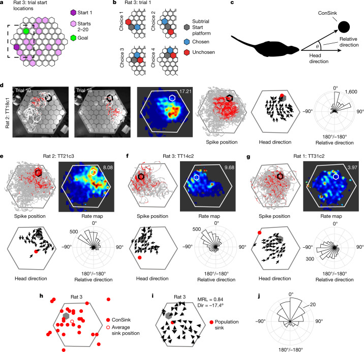
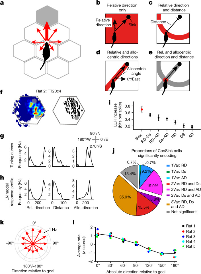
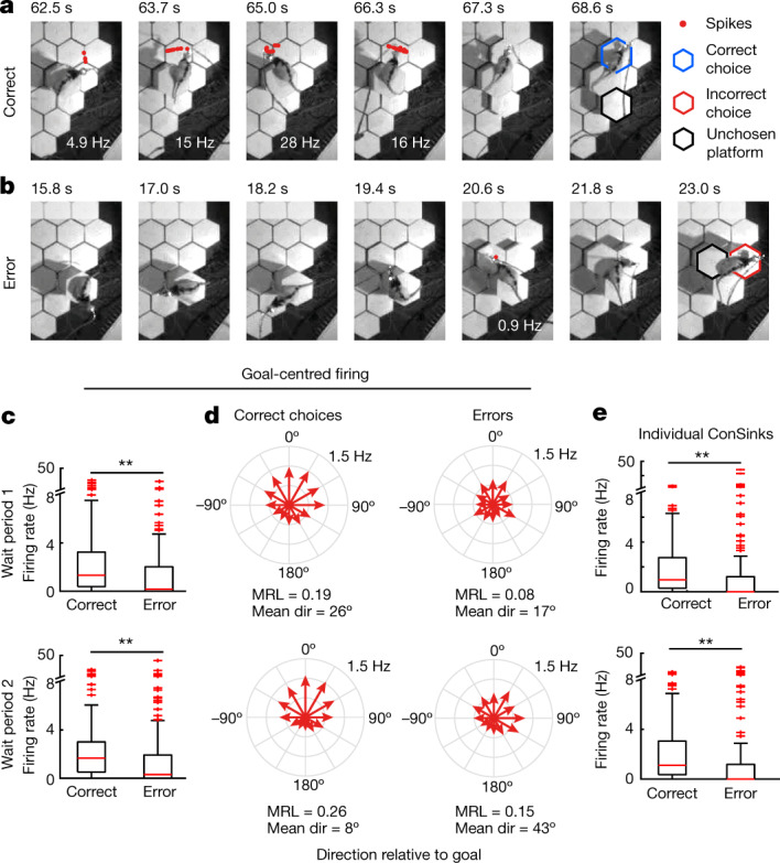
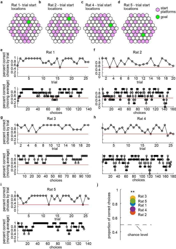
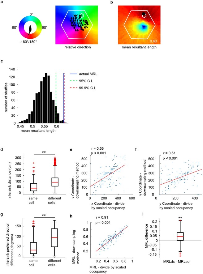
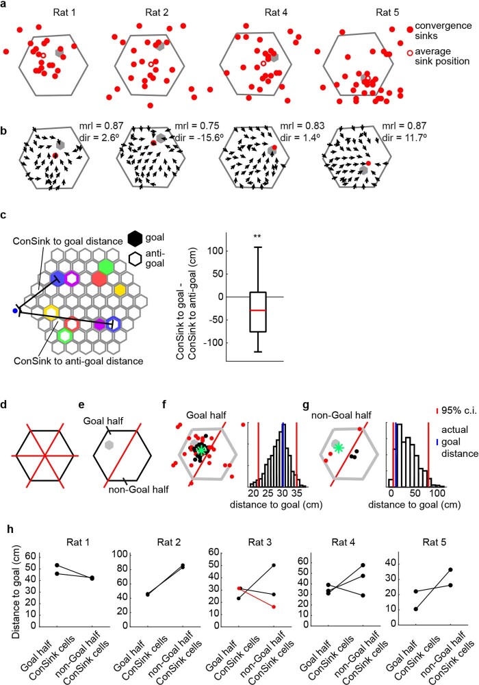
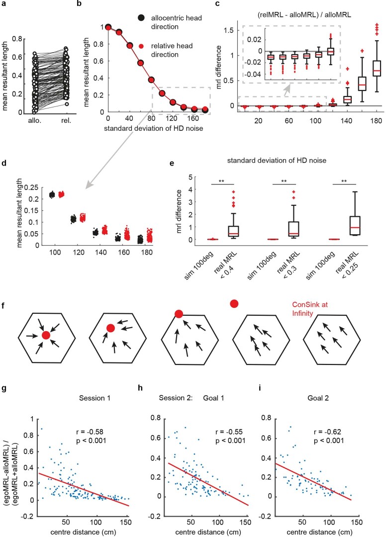
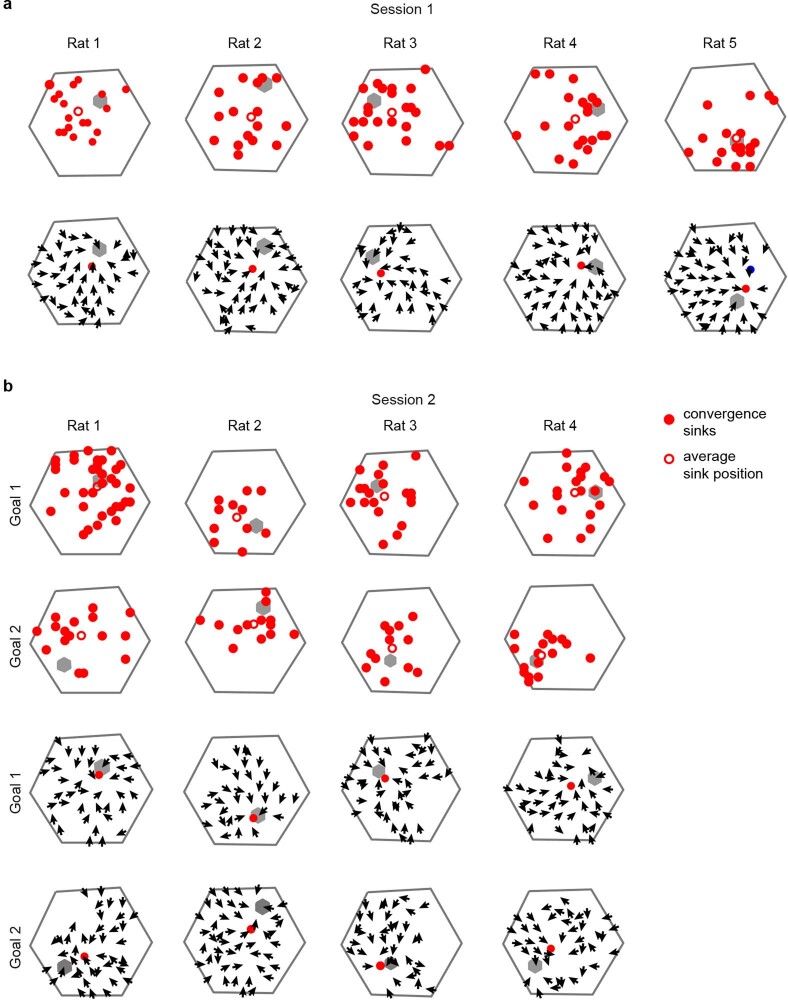
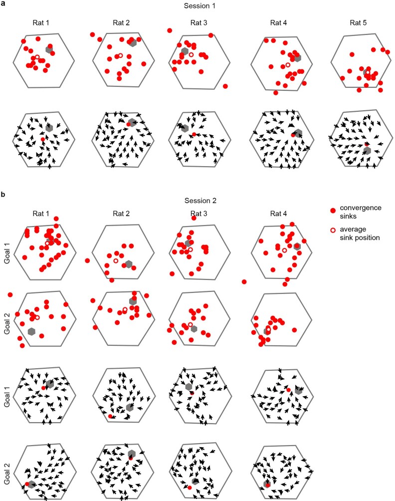
The hippocampal cognitive map supports navigation towards, or away from, salient locations in familiar environments¹. Although much is known about how the hippocampus encodes location in world-centred coordinates, how it supports flexible navigation is less well understood. We recorded CA1 place cells while rats navigated to a goal on the honeycomb maze². The maze tests navigation via direct and indirect paths to the goal and allows the directionality of place cells to be assessed at each choice point. Place fields showed strong directional polarization characterized by vector fields that converged to sinks distributed throughout the environment. The distribution of these 'convergence sinks' (ConSinks) was centred near the goal location and the population vector field converged on the goal, providing a strong navigational signal. Changing the goal location led to movement of ConSinks and vector fields towards the new goal. The honeycomb maze allows independent assessment of spatial representation and spatial action in place cell activity and shows how the latter relates to the former. The results suggest that the hippocampus creates a vector-based model to support flexible navigation, allowing animals to select optimal paths to destinations from any location in the environment.

Fig. 1. ConSinks and vector fields organize place cell activity during navigation on the honeycomb maze.

a, Maze showing all start platforms and the goal platform for rat 3. The dashed box indicates the portion of the maze shown in b. b, Schematic of the four choices making up trial 1. The animal is confined at the ‘subtrial start’ until two adjacent platforms are raised and makes its choice by moving onto the ‘chosen’ platform. c, The animal’s heading direction relative to a reference point (the ConSink) is calculated as the angle between the straight-ahead head direction (0°) and the direction of the point in egocentric space. d, Representative example of a ConSink place cell. Left two panels, paths (white) and spikes (red) fired during two individual trials of the task. The perimeter of the goal platform is shown in black. Middle two panels, place field heat map (maximal firing rate (Hz) indicated at top right) and all paths (grey) and spikes (red). Second from right, vector field depicting mean head direction at binned spatial positions. The ConSink is depicted as a filled red circle. Right, polar plot showing the distribution of head directions relative to the ConSink. e–g, Additional examples as in d. h, ConSinks from rat 3 plotted over the maze showing a wide distribution across and off the maze (see Extended Data Fig. 6a for results from the other four animals). A grey hexagon represents the goal platform. i, Average vector fields for rat 3 (see Extended Data Fig. 6b for results from the other four animals). MRL, mean resultant length; Dir, mean relative direction. j, The mean relative directions of all significant ConSinks were non-uniformly distributed (Rayleigh test: z = 22.19, P = 9.81 × 10⁻¹¹), with a mean direction of −6.20° (not significantly different from 0° (one-sample test for mean angle, P < 0.05); 95% confidence interval = −10.3º, 22.67º). Source Data

Fig. 2. ConSinks are under the influence of goal location.

a, Spatial distribution of ConSinks from rat 3 active only in goal 1 (grey hexagon) before the goal switch. An open circle represents the average ConSink. Results for the remaining animals are shown in Supplementary Fig. 3a–c. b, The ConSink population was significantly closer to goal 1 than to goal 2 before the goal switch (Wilcoxson rank-sum test, one sided: n = 109 cells from four animals, z = −6.85, P = 3.62 × 10⁻¹²). c, Spatial distribution of ConSinks active only in goal 2 (red hexagon) after the goal switch. d, The ConSink population was closer to goal 2 than goal 1 (Wilcoxson rank-sum test, one sided: n = 81 cells from four animals, z = −4.61, P = 1.99 × 10⁻⁶). e, Movement of ConSinks from goal 1 to goal 2 (indicated by arrows). f, ConSinks in e and Supplementary Fig. 3c were closer to the new goal after the switch (Wilcoxson signed-rank test, two sided: n = 28 cells from four animals, z = −2.48, P = 0.013). g,h, Population vector fields for significant ConSink cells during goal 1 (g) and goal 2 (h) for rat 3 (results for the remaining animals are shown in Supplementary Fig. 4). Population sink positions are shown as a red filled circle. i, MRL values taken from MRL maps (Supplementary Fig. 4) at the goals during both epochs (n = 4 animals). MRL values are always highest at the current goal. For all box plots, the central mark indicates the median and the bottom and top edges of the box indicate the 25th and 75th percentiles, respectively; the whiskers extend to the most extreme data points within 1.5 times the interquartile range from the bottom or top of the box, and all more extreme points are plotted individually using a plus symbol. *P < 0.05; **P < 0.001. Source Data

Fig. 3. ConSink population firing patterns contain enough spatial information to solve the honeycomb maze navigation problem.

a, A simple fantail model predicts that firing rate vectors will be maximum in the direction of the goal and fall off monotonically with increasing angle from the goal. b–e, The information necessary to construct the goal direction vector consists of all or certain combinations of the relative direction (b) and distance (c) to the ConSink and absolute direction relative to the environment (d), which together produce the goal direction vector (e). f–h, Typical CA1 place cell with significant information coding for all three variables with raw tuning curves (g) and LN model response profiles (h). i, For the cell in f, the combination of all three types of information provides more information than any other combination (LLH, log-likelihood; 3Var, 3 variables; RD, relative direction; Ds, distance; AD, allocentric direction). n = 10 repeats of the cross-validation procedure. Error bars, s.e.m. j, Percentages of ConSink cells encoding different combinations of the three variables in the LN model. k, Fantail data: population firing rate vectors across the five animals (red arrows) varying monotonically as a function of the angle between each platform direction and the population goal vector (Rayleigh test of non-uniformity of distribution, P = 0; mean direction = 10.9º). l, Population vectors for each animal conform to this model. Individual points correspond to the fantail vectors from each animal; note that positive and negative directional (for example, 30º and –30º) vectors are averaged. The black line represents the average across the five animals. Source Data

Fig. 4. Goal-centred firing by ConSink cells is reduced on error subtrials.

a, Example ConSink cell (rat 2, cell TT18c1, trial 16) immediately before a correct choice. Note the side-to-side scanning and robust firing in the goalward direction before the move onto the correct platform (goal beyond the top of the frame). b, Same cell as in a before an incorrect choice. c, Firing rates in the goalward direction were reduced on error trials, during both wait period 1 (the 4-s period before raising the choice platforms; top) and wait period 2 (the 4-s period before movement onto the chosen platform; bottom). Wilcoxson signed-rank test, two sided: n = 142 cells from five rats, z = 5.61, P = 1.97 × 10⁻⁸ (wait period 1); z = 4.87, P = 1.14 × 10⁻⁶ (wait period 2). d, Fantail plots of firing rates in directions relative to goal during correct choices have canonical forms, as in Fig. 3k, and peaks much closer to 0º than during incorrect choices. e, The tuning of ConSink cells to their individual sink positions is also disrupted on incorrect choices. Wilcoxson signed-rank test, one sided: n = 142 cells from five rats, z = 3.27, P = 5.46 × 10⁻⁴ (wait period 1); z = 3.88, P = 5.17 × 10⁻⁵ (wait period 2). For box plots in c and e, the central mark indicates the median and the bottom and top edges of the box indicate the 25th and 75th percentiles, respectively; the whiskers extend to the most extreme data points within 1.5 times the interquartile range from the bottom or top of the box, and all more extreme points are plotted individually using a plus symbol. **P < 0.001. Source Data

Extended Data Fig. 1. Behavioural Summary.

a, Schematic of the honeycomb maze showing all start platforms and the goal platform from Rat 1’s session. b-d, Same as is in (a) but for Rats 2, 4, and 5, respectively. e, Top panel, Percentage of choices that were correct averaged by trial for Rat 1. Bottom panel, Running average of correct choices (every 5 consecutive choices). f-i, As in (e) but for Rats 2 to 5, respectively. j, The total proportion of correct choices for each rat. Each rat made significantly more correct than incorrect choices; two-sided binomial test within each animal, p = 5.17 x 10⁻⁵, 1.03 x 10⁻⁵, 5.96 x 10⁻¹⁵, 1.32 x 10⁻⁴, 9.16 x 10⁻¹⁶ for rats 1–5, respectively. Source Data

Extended Data Fig. 2. Typical behaviour and spiking of a ConSink neuron.

a, Screengrabs of a complete trial of the honeycomb task (Rat 1, trial 3). In white is the path of the animal from the time of the previous screengrab (or from 0 s for the first screengrab) to the time of the current screengrab. In red are the spikes fired by a representative ConSink cell (TT15c6). b, Screengrabs from a portion of the same trial in (a) at a higher temporal resolution. Note how the animal completes a full 360° rotation while waiting for the next pair of platforms to be presented (platforms start to rise at 142sec); this is typical of all 5 animals’ behaviour. 3 ellipses are drawn over the animal’s cervical (yellow), thoracic (green), and lumbar (blue) regions to show his position and orientation. c, The same cell’s vector field (left) and the polar plot of spike directions relative to the convergence sink (right; the sink is plotted in red at left).

Extended Data Fig. 3. Rats sample a large range of possible directions while navigating the honeycomb task.

a, Histogram showing the directional range covered by the animals per choice from the time when the platforms begin to rise to the time when the animal moves to the next platform. Note that ranges greater than 360º indicate that the animal continued to scan in the same direction (i.e. multiple rotations); if an animal scanned 360º and then counter-rotated back to the starting direction, range is calculated only as 360º. b, Allocentric (allo.) and relative-to-goal (goal) directional occupancy for each animal. Note that goal direction is not oversampled. c, The time the animals take to make their decision decreases as they get closer to goal (one sample t test, t(723) = 6.27, p = 5.94 x 10⁻¹⁰); however, this does not seem to prevent them sampling the full range of direction at short-goal distances (d). Source Data

Extended Data Fig. 4. Histology showing tetrode position in the CA1 cell layer in dorsal hippocampus.

Example cresyl violet stained coronal slices showing tetrode marking lesions in all 5 experimental subjects (Rat 1 (a), 2 (b), 3 (c), 4 (d), and 5 (e)). Scale bar = 1000 µm.

Extended Data Fig. 5. Calculation of the ConSink.

a, Left, each division of the colour wheel represents 1 search position in a polar co-ordinate framework centred on the animal’s head with 0° straight ahead. Right, the spatial environment is tiled by candidate sink positions. At each candidate position, the direction of all spikes relative to that position can be calculated (by subtracting the direction of the vector from the animal to the candidate position from the animal’s allocentric head direction). From this, a mean direction can be calculated, and is plotted here according to the colour wheel at left. The vector field (i.e. the mean allocentric direction of spikes at binned spatial positions) of an example ConSink cell (Rat 2, cell TT18c1) is overlaid. b, At each candidate sink position, the mean resultant length (MRL) of the associated distribution of relative directions is calculated (candidate positions are colour coded by MRL value). The candidate position with the largest MRL, which indicates the concentration of the polar distribution in the mean direction for that position, is taken as the ConSink (black closed circle; MRL = 0.63). c, To determine whether a cell was significantly modulated by relative direction to the candidate position identified as in (b), we shuffled the allocentric head directions associated with each spike, and recalculated relative direction MRLs at each search position, using the maximal MRL for our control distribution. This procedure was repeated 1000 times, and confidence intervals constructed. A cell was deemed to be significantly modulated if it’s MRL was greater than the 95^th percentile of the shuffled distribution of maximal MRLs. d, To confirm the validity of our calculations, we recalculated the sinks in our identified ConSink cells using a downsampling method, in which, for each cell on each platform, the spikes were downsampled according to the directional occupancy in allocentric coordinates (see Methods). We then compared the distances between the sinks calculated with the 2 different methods (our “divide by scaled occupancy” method, and “downsampling” method) within and between cells. We found that sink positions were more similar within cells than across cells (Wilcoxson rank sum test, two-sided, n = 142 cells (same cells) or 20,022 pairs of cells (different cells) from 5 animals, z = −10.04, p = 9.94 x 10⁻²⁴), and x (e, Pearson correlation, r = 0.55, p = 1.50 x 10⁻¹²) and y coordinates (f, Pearson correlation, r = 0.51, p = 1.02 x 10⁻¹²) were strongly correlated across the two techniques. g, Similarly, preferred relative direction was more similar within cells (Wilcoxson rank sum test, two-sided, n = 142 cells (same cells) or 20,022 pairs of cells (different cells) from 5 animals, z = −9. 65, p = 5.07 x 10⁻²²). h, The strength of tuning was also highly correlated between the two techniques (Pearson correlation, r = 0.91, p = 7.99 x 10⁻⁵⁵). i, Lastly, we found that our technique did not overestimate the strength of tuning, as tuning was slightly, but significantly, stronger in the downsampled data (Wilcoxson signed rank test, two-sided, n = 142 cells from 5 animals, z = 5.60, p = 2.18 x 10⁻⁸). For box plots in (d), (g) and (i), the central mark indicates the median, and the bottom and top edges of the box indicate the 25th and 75th percentiles, respectively; the whiskers extend to the most extreme data points within 1.5 times the interquartile range away from the bottom or top of the box, and all more extreme points are plotted individually using the ‘+’ symbol. Source Data

Extended Data Fig. 6. ConSinks cluster around the goal.

a, ConSinks from Rat 1, 2, 4 and 5 plotted over the maze showing that conSinks are widely distributed across the maze, and some are also located past the maze perimeter (see Fig. 1 for Rat 3). Grey hexagons represent goal platforms. b, Average vector fields for Rat 1, 2, 4, and 5 (see Fig. 1 for Rat 3). “mrl”, mean resultant length; “dir”, mean relative direction. c, Left, Schematic of the maze showing positions of goals (red: Rat 1; green: Rat 2; blue: Rat 3; yellow: Rat 4; purple: Rat 5) and platforms used as anti-goals in the analysis at Right. The anti-goal positions were produced by mirroring the goal positions across the axis perpendicular to a line between the maze vertex closest to the goal and the opposite vertex. For each relative direction cell, the distances from its convergence sink to the goal and anti-goal were calculated. The differences between these distances is plotted at Right. Convergence sinks were closer to the goal than the anti-goal, suggesting greater density around the goal (Wilcoxon signed rank test, two-sided, n = 142 cells from 5 animals, z = −4.92, p = 8.61 x 10⁻⁷. For box plot, the central mark indicates the median, and the bottom and top edges of the box indicate the 25th and 75th percentiles, respectively; the whiskers extend to the most extreme data points away from the bottom and top of the box). d, To determine whether clustering around the goal was due to place field locations (taken as the centre of mass), the maze was divided into 2 halves along 3 different axes, producing 3 pairs of halves. e, The half containing the goal is referred to as the “Goal half”, the other as the “non-Goal-half” (for Rats 1, 2, and 5, one pair of halves is eliminated from the analysis as their goals lie on 1 of the 3 axes). f, Left, the place cell positions of the Goal half cells corresponding to the split axis (red line) from Rat 3 shown as black filled circles. The ConSink positions of the same cells shown as red filled circles. The average ConSink position shown as a green asterisk. Goal in grey. Right, Histogram of average ConSink distances to goal calculated by randomly sampling the same number of cells as shown at left, but from the whole maze, repeated 1000 times. The red bars delimit the 95% confidence interval. The goal distance of the average ConSink at left is shown in blue. g, Same as f, but for the non-goal half. h, The distances to goal of each of the 2 or 3 pairs of Goal-half and non-Goal-half average ConSinks for all 5 rats. Note that the significance of the difference for each pair of points was calculated using the bootstrap method shown in (d) and (e); none fell outside the 95% confidence intervals. n = 2 (rats 1, 2 and 5), 3 (rats 3 and 4). Source Data

Extended Data Fig. 7. ConSinks move closer to the original goal with experience within a day.

Compared to ConSinks calculated during the first half of the first recording session (a), ConSinks calculated during the second half of the first session (b) appear more concentrated around the goal. c, Most ConSinks move towards the goal. Arrowheads refer to locations of ConSinks in (b), tails to ConSinks in (a). d, The second half ConSinks are significantly closer to the goal than first half ConSinks (Wilcoxon signed rank test, two-sided, n = 142 cells from 5 animals, z = 3.63, p = 2.86 x 10⁻⁴. For box plot, the central mark indicates the median, and the bottom and top edges of the box indicate the 25th and 75th percentiles, respectively; the whiskers extend to the most extreme data points away from the bottom and top of the box). Source Data

Extended Data Fig. 8. Tuning to the ConSink is not an artefact of allocentric tuning in ConSink cells Part 1.

a, MRLs calculated from allocentric (allo.) and relative (rel.) head directions for each ConSink cell during task. Note that for every ConSink cell, the MRL calculated from relative directions is greater than the MRL calculated from allocentric head directions. n = 142 cells from 4 animals. b-e, Noise in a purely allocentric head direction signal can’t explain the greater egocentric MRLs in ConSink cells. b, We simulated purely allocentric cells by assigning new head direction values to the spikes fired by each ConSink cell. These head directions were calculated by using a given cell’s true mean allocentric head direction and adding increasing levels of noise. We then calculated both allocentric and egocentric MRLs as was done for our real data. In these simulated allocentric cells, egocentric MRLs closely tracked allocentric MRLs, and both decreased with increasing levels of head direction noise. c, Only at noise levels above 100deg standard deviation do egocentric MRLs become larger than allocentric MRLs. n = 142 cells from 5 animals. d, The MRLs at 120deg noise and above were smaller than any we observed in our identified ConSink cells, and thus irrelevant. e, Only in cells with ~100deg of head direction noise, and therefore MRLs of ~0.2 length, would we expect true allocentric cells to have relatively larger egocentric MRLs within the range of values we observed in our data. However, the differences in egocentric MRLs relative to allocentric MRLs in our most weakly tuned ConSink cells were still much greater than could be explained by noise in a purely allocentric signal (Wilcoxon rank sum test, two-sided; left: n = 42 cells from 5 animals, z = −7.89 p = 3.12 x 10⁻¹⁵; middle: n = 24 cells from 5 animals, z = −5.93, p = 3.06 x 10⁻⁹; right: n = 9 cells from 5 animals, p = 4.11 x 10⁻⁵). f, Schematic showing how egocentric tuning appears more allocentric with increased ConSink centre-distance; this is due to the animal’s narrow sampling of allocentric direction when oriented in the cell’s optimal egocentric direction. This leads to the prediction that if ConSink cells are truly tuned to egocentric direction, the difference between the calculated strength of their egocentric and allocentric tunings (see (a)) will decrease with distance from the centre of the maze. g-i, There was a strong negative correlation between egocentric-allocentric tuning difference and distance to the maze centre in both session 1 and session 2 (g, session 1, Pearson correlation, r = −0.58, p = 2.86 x 10⁻¹⁴; h, session 2-goal 1, Pearson correlation, r = −0.55, p = 7.98 x 10⁻¹⁰; i, session 2-goal 2, Pearson correlation, r = −0.62, p = 4.82 x 10⁻¹⁰). For box plots in (c) and (e), the central mark indicates the median, and the bottom and top edges of the box indicate the 25th and 75th percentiles, respectively; the whiskers extend to the most extreme data points within 1.5 times the interquartile range away from the bottom or top of the box, and all more extreme points are plotted individually using the ‘+’ symbol. Source Data

Extended Data Fig. 9. Tuning to the ConSink is not an artefact of allocentric tuning in ConSink cells Part 2.

a, b, Because it is more difficult to distinguish whether cells with sinks off the maze were egocentric or allocentric, we recalculated mean sink positions and population field vectors using only ConSink cells with sinks on the maze (a, Session 1, b, Session 2; number of cell omitted: rat 1, session 1: 3/21; session 2 goal 1: 8/47, goal 2: 9/25; rat 2, session 1: 10/27; session 2 goal 1: 3/14, goal 2: 8/21; rat 3, session 1: 7/29; session 2 goal 1: 4/23, goal 2: 4/16; rat 4, session 1: 8/30; session 2 goal 1: 4/25, goal 2: 3/19; rat 5, session 1: 17/35). Mean sinks continued to move with the goals and field vectors continued to point to the goals.

Extended Data Fig. 10. Tuning to the ConSink is not an artefact of allocentric tuning in ConSink cells Part 3.

a, b, We repeated this analysis omitting those cells with a normalized egocentric-allocentric MRL difference of 0.05, that is, those ConSink cells most likely to be mis-identified as allocentric-tuned cells (number of cells omitted: rat 1, session 1: 6/21; session 2 goal 1: 13/47, goal 2: 8/25; rat 2, session 1: 10/27; session 2 goal 1: 3/14, goal 2: 5/21; rat 3, session 1: 10/29; session 2 goal 1: 3/23, goal 2: 1/16; rat 4, session 1: 7/30; session 2 goal 1: 1/25, goal 2: 2/19; rat 5, session 1: 16/35). Similarly, there was little change in the mean sinks or the field vectors.

References

1. O’Keefe, J. & Nadel, L. The Hippocampus as a Cognitive Map (Oxford University Press, 1978).
1. Wood RA, et al. The honeycomb maze provides a novel test to study hippocampal-dependent spatial navigation. Nature. 2018;554:102–105. doi: 10.1038/nature25433. - DOI - PMC - PubMed
1. Morris RG, Garrud P, Rawlins JN, O’Keefe J. Place navigation impaired in rats with hippocampal lesions. Nature. 1982;297:681–683. doi: 10.1038/297681a0. - DOI - PubMed
1. O’Keefe J, Dostrovsky J. The hippocampus as a spatial map. Preliminary evidence from unit activity in the freely-moving rat. Brain Res. 1971;34:171–175. doi: 10.1016/0006-8993(71)90358-1. - DOI - PubMed
1. O’Keefe J. Place units in the hippocampus of the freely moving rat. Exp. Neurol. 1976;51:78–109. doi: 10.1016/0014-4886(76)90055-8. - DOI - PubMed