A transcriptomic axis predicts state modulation of cortical interneurons

Abstract

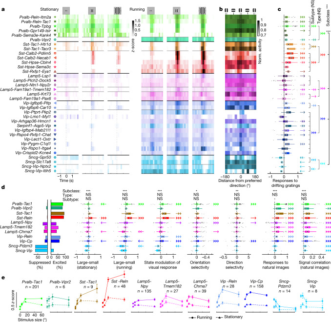
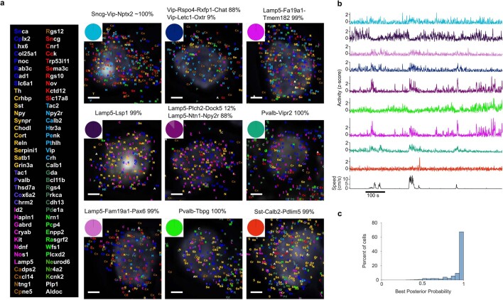
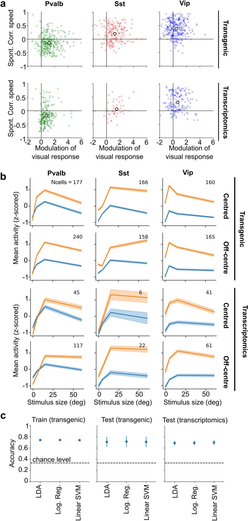
Transcriptomics has revealed that cortical inhibitory neurons exhibit a great diversity of fine molecular subtypes^1-6, but it is not known whether these subtypes have correspondingly diverse patterns of activity in the living brain. Here we show that inhibitory subtypes in primary visual cortex (V1) have diverse correlates with brain state, which are organized by a single factor: position along the main axis of transcriptomic variation. We combined in vivo two-photon calcium imaging of mouse V1 with a transcriptomic method to identify mRNA for 72 selected genes in ex vivo slices. We classified inhibitory neurons imaged in layers 1-3 into a three-level hierarchy of 5 subclasses, 11 types and 35 subtypes using previously defined transcriptomic clusters³. Responses to visual stimuli differed significantly only between subclasses, with cells in the Sncg subclass uniformly suppressed, and cells in the other subclasses predominantly excited. Modulation by brain state differed at all hierarchical levels but could be largely predicted from the first transcriptomic principal component, which also predicted correlations with simultaneously recorded cells. Inhibitory subtypes that fired more in resting, oscillatory brain states had a smaller fraction of their axonal projections in layer 1, narrower spikes, lower input resistance and weaker adaptation as determined in vitro⁷, and expressed more inhibitory cholinergic receptors. Subtypes that fired more during arousal had the opposite properties. Thus, a simple principle may largely explain how diverse inhibitory V1 subtypes shape state-dependent cortical processing.

Fig. 1. Post-hoc transcriptomic identification of recorded neurons.

a, Three-dimensional (3D) representation of an example reference z-stack (white: GCaMP6m, expressed in all neurons, red: mCherry, expressed in inhibitory neurons) . b, Digital sagittal section of this z-stack (maximum intensity projection, 15-μm slice); colours as in a. Scale bar, 100 µm. c, Portion of ex vivo slice aligned to section in b after 72-fold mRNA detection with coppaFISH. Dots represent detected mRNAs (colour code: top of i). Scale bar, 100 µm. d, Expanded view of dashed rectangle in b,c showing in vivo mCherry fluorescence (red) and ex vivo Gad1 mRNA detection (blue). Scale bar, 20 µm. e, mRNAs detected in this same region, plotted as in c. White lines indicate two functional imaging planes. Grey background: DAPI stain for cell nuclei. Scale bar, 20 µm. f, Hierarchical classification of in-vivo-recorded cells into 5 subclasses, 11 types and 35 subtypes. Within each type, subtypes are sorted by their mean first transcriptomic principal component (tPC1) score (see Fig. 5b). Lect1 is also known as Cnmd; Fam19a1 is also known as Tafa1. g, Higher-magnification view of cells 1 and 2 from e. Gene detections are indicated by coloured letters (code: top of i). Grey background: DAPI image. Below: pie charts indicating probabilities of assignment to subtypes. Scale bars, 5 µm. h, Deconvolved calcium traces for the two example cells, together with running speed. i, Mean expression of the 72 genes (pseudocoloured as log(1 + gene count)) for the 35 subtypes, ordered as in f (n = 4 mice). Left: number of unique cells of each subtype. Nov is also known as Ccn3. j, Comparison of the median cortical depth of each subtype found using coppaFISH (as a fraction of total depth; n = 14 sections from a brain in which mRNAs were detected down to layer 6), and its median cortical depth found independently using Patch-seq (Pearson correlation: r = 0.91, P = 1 × 10⁻¹³; analysis of covariance (ANCOVA) controlling for subclasses and types: F(1) = 163.6, P = 6 × 10⁻¹²). Only subtypes with at least four cells for each dataset were considered. Symbols for subtypes imaged in vivo are shown in f; for subtypes too deep to image, symbols are shown on the right. Source data

Fig. 2. Example raster of spontaneous neuronal activity.

Raster of spontaneous neuronal activity (grey screen) for an example session. a, Running speed, pupil size and mean activity of the 10% of excitatory cells (ECs) with most negative principal component weights (oscillation). b, Raster of EC activity, sorted by weight on the first principal component of their activity. c, Raster of the activity of inhibitory cells (ICs), grouped and coloured by subtype. The three columns on the right show an expanded view of the time windows marked in a, illustrating three behavioural states. These rasters show all recorded ECs (413 cells) and molecularly identified ICs (117 cells) in this session (94 ICs not matched to in situ transcriptomics are not shown; note the different scale bars for ECs and ICs). Neuronal activity was z-scored and then smoothed with a 1-s boxcar window. Source data

Fig. 3. State modulation of inhibitory subtypes.

a, Nested permutation analysis for spontaneous correlations. Top, significance of omnibus test for higher correlations within subclasses (P < 0.0001), nested types (P < 0.0001) and subtypes (P = 0.048). Right bolded brackets: significant post-hoc tests within each grouping (Benjamini–Hochberg-corrected; P values in Extended Data Fig. 6b). b, Left, pseudocolour representation of the mean activity of each subtype in each state. Middle, box plots showing the distributions of state modulation (running versus stationary synchronized) for cells of each subtype (n = 4 mice, 17 sessions; for box definitions, see Methods). Right, nested permutation analysis, plotted as in a. Omnibus test found significantly different state modulation between subclasses (P < 0.0001), nested types (P = 0.022), and subtypes (P = 0.014). Benjamini–Hochberg-corrected post-hoc tests found significant differences within Pvalb (P < 0.0001), Sst (P < 0.0001), Lamp5 (P = 0.0025), Vip (P < 0.0001) and Lamp5-Npy (P < 0.0001) cell groups. Coloured arrows at each level indicate significant state modulation for each cell group (two-sided t-tests, Benjamini–Hochberg-corrected; number of arrowheads indicates significance). c, Modulation for running versus stationary desynchronized states, against modulation for stationary synchronized versus desynchronized states. Each glyph shows mean values for a subtype; symbols as in b (F(1) = 375.4, P = 3.6 × 10⁻⁷¹, ANCOVA controlling for session). d, Modulation for running versus stationary desynchronized states against locking to the synchronized state oscillation. Each glyph shows mean values for a subtype (F(1) = 240.5, P = 2 × 10⁻⁴⁷, ANCOVA controlling for session). e, State modulation for cells in the Lamp5-Plch2-Dock5 and Lamp-Lsp1 subtypes, against subtype probability index (log(P_Subtype1/P_Subtype2); left), or Ndnf (middle) and Cck (right) gene expression. These three variables correlated significantly with state modulation (Pearson correlation: subtype probability: P = 2 × 10⁻⁷, r = −0.39; Ndnf expression: P = 2 × 10⁻⁵, r = 0.32; Cck expression: P = 2 × 10⁻⁴, r = −0.29), even controlling for a common effect of subtype (F(1) = 4.8, P = 0.03; F(1) = 6.2, P = 0.014; F(1) = 10.7, P = 0.0014, respectively, ANCOVA). Black lines: linear fits. *P < 0.05, **P < 0.01, ***P < 0.001; one-, two- or three-headed arrows in c indicate the same significance levels; direction indicates the sign of modulation. Source data

Fig. 4. Sensory responses of inhibitory subtypes.

a, Pseudocolour activity rasters trial-averaged on the onset of drifting grating stimuli (duration 0.5 s), for different stimulus sizes (5°, 15° and 60°) and locomotor states. Each row shows the average activity of a subtype. Dashed grey lines: stimulus onset. b, Cross-validated direction tuning curves for each subtype, shown in pseudocolour as a function of grating direction. Tuning curves were averaged over odd trials, and shifted relative to the preferred direction found on even trials; thus, a peak will only appear at 0 if the cell is genuinely tuned. c, Nested permutation analysis of drifting grating responses (measured at the stimulus size eliciting the largest negative or positive response), plotted as in Fig. 3b. Top, significance of omnibus test for differences between subclasses (P < 0.0001) and nested types (P = 0.99) and subtypes (P = 0.49). d, Additional analyses of stimulus responses. From left: fraction of cells of each type significantly excited or suppressed by grating stimuli; hierarchical analyses of response differences between large and small gratings in stationary and running conditions; state modulation of visual response by running, averaged over all sizes; orientation and direction selectivity; and mean response and reliability (signal correlation) for natural image stimuli. Nested permutation analyses plotted as in Fig. 3b but only to type level; full plots and P values are in Extended Data Fig. 7. e, Mean size tuning curves for each type, showing the mean responses in stationary (dashed lines, triangles) and running (solid lines, circles) epochs. Only cells with receptive fields < 20° from the stimulus centre are included. Error bars, s.e.m. (n = 4 mice, 17 sessions; numbers below the type name on each plot indicate the number of cells). *P < 0.05, **P < 0.01, ***P < 0.001; NS, not significant; one-, two- or three-headed arrows in c,d indicate the same significance levels; direction indicates the sign of modulation. Source data

Fig. 5. A single transcriptomic axis predicts state modulation.

a, Loading of each gene onto tPC1. b, Ordering of subtypes by tPC1. Left, original ordering by subclass and type as in previous figures. Middle, subtypes re-ordered by the mean of tPC1. Right, violin plots showing the distribution of tPC1 values over cells of each subtype. c, Correlation between state modulation and tPC1. Each glyph represents mean values for a subtype; symbols as in b (F(1) = 14.5, P = 2 × 10⁻⁴, ANCOVA controlling for session and subclass). d, Matrix of pairwise correlations between simultaneously recorded types. The types are sorted by tPC1, showing a significant effect of tPC1 on the pairwise correlations (P = 0.014; one-sided permutation test). *P < 0.05, ***P < 0.001. Source data

Fig. 6. Correlation of state modulation with cellular properties.

a, Correlation between state modulation and electrophysiological properties measured by an independent Patch-seq study. Each symbol represents mean values for a subtype, coded as in Fig. 5b. Rheobase: r = −0.63, P = 5 × 10⁻⁵; spike adaptation: r = 0.70, P = 3 × 10⁻⁶; spike shape index: r = 0.49, P = 0.003; time constant: r = 0.57, P = 4 × 10⁻⁴ (significance, Pearson correlation). b, Correlation between state modulation and cholinergic receptor expression obtained from an independent scRNA-seq study. Each symbol represents mean values for a given subtype, coded as before. Chrm4: r = −0.50, P = 0.002; Chrm3: r = 0.63, P = 5 × 10⁻⁵; Chrna4: r = 0.52, P = 0.0014; Chrna5: r = 0.37, P = 0.03. Correlations of state modulation with excitatory cholinergic receptor expression were higher than with inhibitory receptor expression (including receptors not shown here; P = 0.008, F(1) = 12.2, two-sided ANOVA; only receptors with more than 2 counts in at least 5 subtypes were considered, making 10 in total). *P < 0.05, **P < 0.01, ***P < 0.001; black lines are linear regression fits. c, Schematic summarizing the transcriptomic axis and its functional and cellular correlates. Right, schematic of inputs from inhibitory neurons along the transcriptomic axis to a layer-2/3 (L2/3) cortical excitatory cell. ACh, acetylcholine. Source data

Extended Data Fig. 1. Detection of 72 genes using coppaFISH.

a, Sagittal 15 µm brain sections are cut using a cryostat. Local mRNAs are reverse transcribed to cDNA, and the mRNAs digested to free the cDNAs for hybridization with padlock probes. Padlock probes have two 15-20-nt arms complementary to the target site, a 20-nt anchor sequence (identical for all probes) and a 20-nt barcode sequence (unique for each gene). After hybridization to the target site, a DNA ligase enzyme circularizes the padlock probe, but only when it matches the target perfectly. Next, a DNA polymerase enzyme amplifies the circularized padlock probes, producing rolling-circle products (RCPs), which contain many repeats of the padlock sequence including the barcode. b, The barcodes are read out by 7 rounds of 7-colour fluorescence imaging. On each round, RCPs are hybridized with custom designed bridge probes, which in turn hybridize to specific dye probes (conjugated to one of 7 fluorophores). The sections are then imaged in 7 colour channels, then all DNA is removed with formamide treatment, and the next round begins. Different sets of bridge probes on each round result in each barcode showing up in a different colour channel using a Reed–Solomon code for minimum overlap. After the 7 combinatorial rounds, a final round images the anchor probe (used for image alignment) and DAPI to visualize cell nuclei. c, Example raw data for one cell imaged with the 7 fluorophores and 7 rounds. Each fluorescent spot is an RCP, and the sequence of colours across 7 rounds allows gene identity to be determined. Bottom: magnification of 2 RCPs (top right corner of main images) which corresponded to Cplx2 barcode (6135024). Scale bars: 5 µm.

Extended Data Fig. 2. Experimental pipeline.

Neural activity was recorded in vivo over multiple sessions from each subject (Gad2-mCherry mice with viral GCaMP6m expression in all neurons). At the end of each session, a high-resolution reference Z-Stack was acquired and used to detect interneurons in the Z-stack volume using mCherry fluorescence, and cells recorded during calcium imaging were registered to this Z-Stack. After all imaging sessions, the brain was extracted from the skull without fixation and frozen in OCT. A block from under the imaging window was sliced into 15 μm sagittal sections, which were thaw-mounted on gelatine-coated coverslips. Each section was then processed using coppaFISH: RCPs were produced in situ for the selected genes, and their barcodes were read using 7 rounds of imaging (+ 1 round of anchor and DAPI staining). The resulting images were then registered across rounds, colour channels, and image tiles and individual spots detected. Gene identity for each RCP was decoded from the 49-dimensional images, and pciSeq was used to determine the subtype probabilities for each cell. To align the images, interneurons detected in vivo and ex vivo were used as fiducial markers for point cloud registration, which finds the best alignment of the 2D ex vivo slice in the 3D volume. Finally, individual cell matches were manually curated, and a subtype assigned to the recorded cells.

Extended Data Fig. 3. UMAP analysis of scRNA-seq data.

Each dot represents a V1 inhibitory cell, from the Tasic et al. data, with glyph representing its assigned subtype. UMAP analysis was performed separately for MGE and CGE derived interneuron subtypes, using 150 log-transformed genes selected by the ProMMT algorithm. This analysis reveals both highly discrete subtypes such as Pvalb-Vipr2 (putative chandelier cells) and smoothly varying continua where boundaries between subtypes appear arbitrary, such as Lamp5-Ntn-Npy2r, Lamp5-Plch2-Dock5, and Lamp5-Lsp1 (putative neurogliaform subtypes). Also note the smooth transition between Sst-Calb2 (putative Martinotti subtypes), Sst-Tac1 (putative Sst non-Martinotti), and Pvalb-Tpbg (putative superficial basket cell subtypes). Text on main plots indicates location of in vivo imaged subtypes. Source data

Extended Data Fig. 4. Example cells.

a, Nine example cells which were recorded during the same session as in Fig. 2. Pie plots indicate the posterior probabilities of each cell’s subtype assignment. Grey background images show DAPI-stained nuclei. Each gene detection is represented by coloured letters (key to the left). Scale bars: 2 µm. b, Activity of these 9 cells during spontaneous behaviour, together with the running speed of the mouse. The traces are colour coded according to the assigned subtype for each cell (pie plots in a). c, Analysis of Bayesian classification confidence. Histogram shows posterior probability for a cell to belong to its assigned subtype, for in vivo imaged cells. About 2% of cells for which confidence was below 50% were not analysed further.

Extended Data Fig. 5. Comparison with results in transgenic mice.

a, Top row: modulation of visual responses by running vs. correlation to running speed during spontaneous behaviour, for Pvalb, Sst, and Vip interneurons identified in transgenic mouse lines. Data re-analysed from Ref. and including 4 new mice. Bottom row: same analysis using interneurons identified by post-hoc transcriptomic analysis (data from this study; the Vip group included Vip-positive Sncg cells which are likely to be labelled in the Vip-Cre transgenic line). b, Size tuning curves of Vip, Pvalb and Sst cells for both datasets. Top row: responses measured in transgenic mice for centred stimuli (0-10° offset from receptive field centre); second row: response to off-centre stimuli (10-20° offset from receptive field) in transgenic mice; bottom two rows, same from post-hoc transcriptomics. Orange curves: responses during running; blue curves, responses during stationary epochs. Numbers at the top right corner of each plot indicate number of cells. Data are given as mean ± s.e.m. c, Classification of cell type from physiological features was identical for the two cell typing methods. Each cell was assigned to either Sst, Pvalb or Vip based on 14 physiological features (such as correlation to running speed, size tuning curves, skewness), using one of 3 different linear classifiers trained on a training set randomly selected from the transgenic recording sessions. Left: training-set classifier accuracy averaged over multiple random selections of the training set. Centre: accuracy of the classifiers averaged over the held-out transgenic sessions (test sets). Right: out-of-sample accuracy of the linear models on data with interneurons identified by post-hoc transcriptomics. Note the similar performance on transgenic and transcriptomic test sets. Error bars: s.d. over divisions into training and test set.

Extended Data Fig. 6. Further analyses of state modulation during spontaneous behaviour.

a, Illustration of nested permutation test method. The test asks whether a quantity of interest differs significantly between cell groups, at each level of the classification hierarchy: whether it differs between subclasses, between types belonging to a single subclass, and between subtypes belonging to a single type. To use the test, one first computes a test statistic (such as the mean correlation coefficient of cells assigned to the same group). To obtain a p-value, this test statistic is compared to a null distribution obtained by shuffling the cells’ transcriptomic labels within the appropriate hierarchical level, in a one-sided manner. To test for a difference between the top-level subclasses, cells are shuffled without restriction (1). To test for a difference between types within subclasses, cells are shuffled separately within each subclass (2). To test for a difference between subtypes within types, cells are shuffled separately within each type (3). In all three cases, cells are only shuffled within experiments, to avoid conflating variability between experiments with variability between cell types. b, Nested permutation test results for pairwise spontaneous correlations. Left: blue histograms represent the probability of observation obtained by shuffling transcriptomic labels 10,000 times at three hierarchical levels (see a). Red lines: observed value of the test statistic. Middle: post-hoc tests for each subclass. Right: post-hoc tests for each type containing at least 2 subtypes. All post-hoc p-values were adjusted with Benjamini–Hochberg correction for multiple comparisons. c, Nested permutation analysis of modulation between running and stationary desynchronized states, plotted as in Fig. 3b. Top: significance of omnibus test for differences between subclasses (p < 0.0001) and nested types (p = 0.21) and subtypes (p = 0.038). Post-hoc p-values were adjusted with Benjamini–Hochberg correction (Pvalb: p < 0.0001, Sst: p < 0.0001, Vip: p < 0.0001, Lamp5-Npy: p < 0.0001) d, Nested permutation analysis of modulation between stationary desynchronized and stationary synchronized states, plotted as in Fig. 3b. Top: significance of omnibus test for differences between subclasses (p < 0.0001) and nested types (p = 0.007) and subtypes (p = 0.088).Post-hoc p-values were adjusted with Benjamini–Hochberg correction (Pvalb: p = 0.0075, Sst: p < 0.0001, Vip: p < 0.0001, Lamp5: p < 0.0001 Lamp5-Npy: p = 0.04) e, State modulation vs. subtype probability index for Sst-Calb2-Necab1 and Sst-Calb2-Pdlim5 cells, plotted as in Fig. 3e (Pearson correlation: r = 0.43, p = 0.005; ANCOVA accounting for effects of subtype: F(1) = 7.3, p = 0.011). *, p < 0.05, **, p < 0.01, ***, p < 0.001; 1, 2, or 3-headed arrows in c and d indicate same significance levels, direction indicates the sign of modulation. Source data

Extended Data Fig. 7. Further analyses of visual responses.

Each panel shows a nested permutation analysis for the visual variables analysed in Fig. 4d, but extended to the subtype level. All panels plotted as in Fig. 3b. Post-hoc comparisons of multiple cell groupings are Benjamini–Hochberg corrected within each of these plots. Omnibus and post-hoc tests hierarchical permutation tests are one-sided, one-sample post-hoc t-tests are two-sided. a, Response differences between large and small gratings in stationary periods (subclass: p < 0.0001; Post-hoc tests: Vip-Cp: p = 0.036). b, Response differences between large and small gratings during running (subclass: p < 0.0001; Post-hoc tests: Lamp5: p = 0.04). c, State modulation of visual response by running, averaged over all sizes (subclass: p < 0.0001). d, Orientation selectivity (subclass: p = 0.02). e, Direction selectivity (subclass: p = 0.001). f, Mean response for natural image stimuli (subclass: p < 0.0001; subtype: p = 0.037; Post-hoc tests: Lamp5: p= < 0.0001, Sst: p = 0.01). g, Reliability (signal correlation) for natural image stimuli (subclass: p < 0.0001; Post-hoc tests: Lamp5: p = 0.015). *, p < 0.05, **, p < 0.01, ***, p < 0.001; 1, 2, or 3-headed arrows indicate same significance levels, direction indicates the sign of modulation. Source data

Extended Data Fig. 8. Additional analyses of the relationship between tPC1 and state modulation or pairwise correlations.

a, Correlation of state modulation with natural log expression of two individual genes, Slc6a1 and Gad1, plotted as in Fig. 5c. (ANCOVA controlling for session, F(1) = 138.2, p = 6×10⁻³⁰; F(1) = 50.7, p = 2×10⁻¹², respectively) b, Variance fraction of a cell’s state modulation explainable by successive transcriptomic dimensions. Blue points: fraction of cross-validated variance explainable by multiple linear regression from successive transcriptomic PCs. Dashed lines: fraction of variance explainable by discrete classification according to a cell’s subtype, type or subclass assignment. The first transcriptomic PC explains respectively 70%, 79% and 108% of the variance explainable by subtype, type and subclass assignment. c, d, e, Pairwise correlations between simultaneously recorded types, plotted as in Fig. 5d, but separately for periods within each of the three states (running, stationary desynchronized, and stationary synchronized). The types are sorted by tPC1; types with similar tPC1 values have significantly higher correlations (one-sided permutation test, p = 0.025, p = 0.038, p = 0.005 respectively). f, The permutation test showing higher correlations amongst cells of similar tPC1 used as test statistic the difference between the average of correlation coefficients close to the diagonal (left), and the average of all other off-diagonal coefficients; intra-type correlations were not used. This test statistic was compared to a null ensemble obtained after shuffling tPC1 values 10,000 times. *, p < 0.05, **, p < 0.01, ***, p < 0.001. Source data

Extended Data Fig. 9. Additional analyses of Patch-seq data.

a, Additional electrophysiological properties vs. State modulation plotted as in Fig. 6a. V_rest: r = 0.49 p = 0.003, Sag: r = 0.19 p = 0.27, τ: r = 0.5 p = 0.002, F-I curve slope: r = 0.53 p = 0.001, V_m for Sag: r = -0.56 p = 5×10⁻⁴, Latency: r = -0.31 p = 0.07, Avg. isi (inter-spike interval): r = 0.46 p = 0.005, Resistance: r = 0.59 p = 2×10⁻⁴, Capacitance: r = 0.05 p = 0.78, log(Capacitance) : r = 0.1 p = 0.64, log(Sag) : r = 0.19 p = 0.3 and log(Latency): r = -0.04 p = 0.8. Stars show significance assessed by Pearson correlation (two-sided tests). Black lines are linear fits. b, Fraction of axonal arborization (measured by surface area) in layer 1 (left) and layer 2-3 (right) vs. tPC1 computed for each Patch-seq neuron. Each symbol represents a cell. Pearson correlation (two-sided tests) was computed individually within each subclass, and p-values were adjusted with Benjamini–Hochberg correction (Layer 1 Lamp5: r = 0.63 p = 4×10⁻⁵; Layer 1 Sst: r = 0.41 p = 0.046; Layer 2-3 Lamp5: r = -0.59 p = 3×10⁻⁴; Layer 2-3 Sst: r = -0.44 p = 0.03). Coloured lines show linear fit for each subclass with significant Pearson correlation. *, p < 0.05, **, p < 0.01, ***, p < 0.001. Source data

Extended Data Fig. 10. Confusion matrices for cell-type classification on subsampled scRNA-seq data.

To evaluate the accuracy of our cell classification algorithms, we generated simulated ground-truth by random subsampling from scRNA-seq data. A simulated coppaFISH gene count was obtained for each cell in the V1 scRNA-seq data of Ref. (5680 cells from 60 GABAergic clusters) by drawing each gene's expression from a Poisson distribution with mean equal to the scRNA-seq read count, divided by a factor of 100 to account for the relative inefficiency of in situ detection. 10-fold cross-validation was used, sequentially using 90% of the cells to compute the mean gene expression per subtype used for classification, and the remaining 10% for evaluation. Cells were classified using the approach taken for coppaFISH data. This procedure was repeated 10 times to estimate the classification accuracy for all 5680 simulated cells. a, b, c, Confusion matrices for classification accuracy at the level of subtypes, types and subclasses using our standard 72-gene panel. Each row shows the results for cells initially classified by Ref. to one subtype, type or subclass, with the size of the circles on that row showing the number of subsampled cells assigned to each subtype, type or subclass using our approach. Subtypes, types and subclasses are assigned correctly with 76.4%, 96.6% and 98.1% accuracy respectively. d,e,f, Using a 150-gene panel (selected by the ProMMT algorithm, same panel used to generate the UMAP of Extended Data Fig. 3) increases performance by only 3.5% over the 72-gene panel for subtype assignment and gave very similar performance for type and subclass. Using a yet larger panel of 6000 genes leads to worse performance than the 72-gene panel, owing to overfitting (not shown; 76.8%, 93.6% and 95.4% accuracy for subtype, type and subclass assignment respectively). Source data

References

1. Callaway EM, et al. A multimodal cell census and atlas of the mammalian primary motor cortex. Nature. 2021;598:86–102. - PMC - PubMed
1. Scala F, et al. Phenotypic variation of transcriptomic cell types in mouse motor cortex. Nature. 2021;598:144–150. - PMC - PubMed
1. Tasic B, et al. Shared and distinct transcriptomic cell types across neocortical areas. Nature. 2018;563:72–78. - PMC - PubMed
1. Paul A, et al. Transcriptional architecture of synaptic communication delineates GABAergic neuron identity. Cell. 2017;171:522–539. - PMC - PubMed
1. Zeisel A, et al. Molecular architecture of the mouse nervous system. Cell. 2018;174:999–1014. - PMC - PubMed
Publication types