Physics-driven coarse-grained model for biomolecular phase separation with near-quantitative accuracy

Abstract

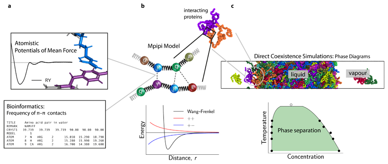
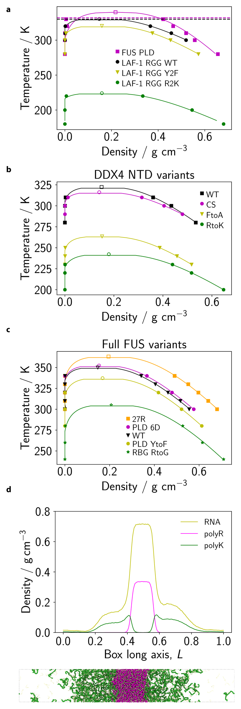
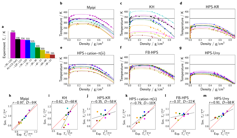
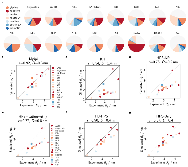
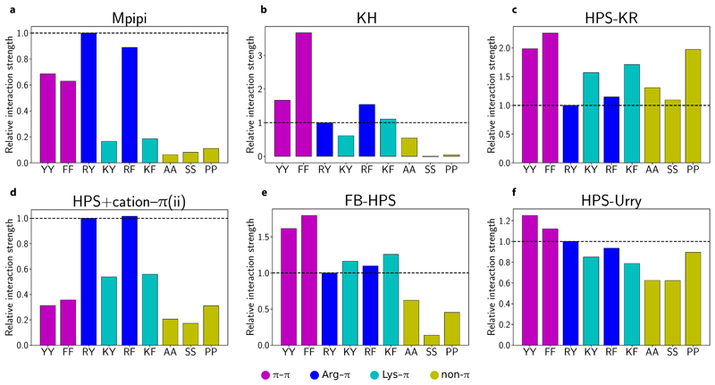
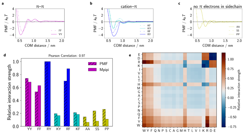
Various physics- and data-driven sequence-dependent protein coarse-grained models have been developed to study biomolecular phase separation and elucidate the dominant physicochemical driving forces. Here, we present Mpipi, a multiscale coarse-grained model that describes almost quantitatively the change in protein critical temperatures as a function of amino-acid sequence. The model is parameterised from both atomistic simulations and bioinformatics data and accounts for the dominant role of π-π and hybrid cation-π/π-π interactions and the much stronger attractive contacts established by arginines than lysines. We provide a comprehensive set of benchmarks for Mpipi and seven other residue-level coarse-grained models against experimental radii of gyration and quantitative in-vitro phase diagrams; Mpipi predictions agree well with experiment on both fronts. Moreover, it can account for protein-RNA interactions, correctly predicts the multiphase behaviour of a charge-matched poly-arginine/poly-lysine/RNA system, and recapitulates experimental LLPS trends for sequence mutations on FUS, DDX4 and LAF-1 proteins.

Figure 1. Designing a coarse-grained model for LLPS from potential-of-mean-force calculations and bioinformatics data.

a (Top) Potential of mean force (PMF) of selected amino-acid (or nucleic-acid) pairs are computed in all-atom simulations with explicit solvent and ions. The computed curves provide a free energy of interaction for the pair in question. (Bottom) The frequencies of π–π contacts for amino acids are obtained from bioinformatics work [13]. Together, these data are used to parameterise the pairwise interactions in the Mpipi model. b (Top) In the Mpipi model, each amino acid (or nucleic acid) is represented by a unique bead. The potential energy is computed as a sum of short-ranged pairwise terms, electrostatic interactions and bonded interactions modelled as harmonic springs. (Bottom) Short-ranged pairwise and electrostatic interactions are computed via a Coulomb term with Debye–Hückel screening (red and blue curves) and the Wang–Frenkel potential [19] (black curve), respectively. c To study biomolecular phase behaviour, we use direct-coexistence molecular-dynamics simulations [20] and compute phase diagrams in the temperature–concentration (or density) space.

Figure 2. Obtaining the correct balance of π–π and non-π-based interactions in the Mpipi model.

a–c PMF calculations at 150 mm NaCl salt concentration for π–π, cation–π and non-π-based interactions, respectively, as a function of the centre-of-mass (COM) distance. Statistical errors (mean±s.d.) are given as error bands, and are only just larger than the line width. They were computed via Bayesian bootstrapping of 3 independent simulations. Each pair is labelled using one-letter amino-acid codes (SI Table I). d Comparison of relative interaction strengths of selected residue pairs (SI Table I) from the PMF calculations with those implemented in the Mpipi model, relative to the Arg–Tyr (RY) interaction. Values are computed by taking the integral of the curves in a–c and the integral of the Wang-Frenkel potential only (between σ and 3σ) for the PMF and Mpipi sets, respectively; for the PMF data only the leftmost well is considered. These correspond to mean energies in the high-temperature limit. e Summary of relative interaction strengths in the Mpipi model. These relative interaction strengths include electrostatic interactions and are computed by numerically integrating Eq. (8) and normalising the result by the RY interaction strength.

Figure 3. Relative contributions of π–π, cation–π and non-π-based interactions in different residue-level models.

a–f Relative interaction strengths [Eq. (8)] for selected residue pairs (see SI Table I for one-letter amino-acid codes) in Mpipi, KH, HPS-KR, FB-HPS, HPS+cation–π(i) and HPS+cation–π(ii) models. For each model, the data set is normalised relative to the corresponding Arg–Tyr (RY) interaction. In each plot, a horizontal dashed line at the RY interaction strength is provided for comparison purposes. Aromatic π–π interactions are coloured in magenta, Arg–π in blue, Lys–π in cyan and non-π-based interactions in dark yellow.

Figure 4. Comparison of single-molecule radii of gyration with experiment.

a Composition of simulated IDPs. We select 17 IDPs for which experimental radii of gyration (R_g) are available (see SI Sec. S2.1 and SI Table III) and assess the composition of the IDPs in terms of the proportion of glycine (orange), neutral (dark yellow; no net charge at pH 7 and no π electrons in side-chain: A, C, I, L, M, P, S, T, V), neutral with π (green; no net charge at pH 7 with π electrons in side chain: N, Q), positive (cyan; without π electrons in side-chain: K), positive with π (blue; with π electrons in side-chain: H, R), negative (red: D, E) and aromatic (magenta: F, W, Y) residues. b–g Comparison of simulated and experiment R_g. R_g values are computed at 300 K in each model. Each protein is coloured based on its dominant residue class (as categorised in a and excluding the ‘neutral’ class). The broken line represents the ‘perfect fit’ line. For each model, the Pearson correlation coefficient r and the root mean squared deviation D are reported in the respective figure title.

Figure 5. Recapitulating the phase behaviour of A1-LCD variants.

a Nine variants of the A1-LCD (including the wild-type) are studied in this work. Variants are prepared following Bremer et al. [10] Experimental critical temperatures are estimated as described in SI Sec. S2.2. The colour of each variant used in panel a is also used in all remaining panels. b–g Phase diagrams for A1-LCD variants obtained via direct-coexistence simulations using the Mpipi, KH, HPS-KR, HPS+cation–π(ii), FB-HPS and HPS-Urry models, respectively. Estimation of critical points of simulated phase diagrams is described in the Methods section. Curves are derived from empirical fits of the data to Eqs (6) and (7); typical errors are discussed in SI Sec. S8.4. h–m Simulated critical temperature T_c relative to the critical temperature of the wild type $(T_c^{wt})$ shown against the experimental analogue. The Pearson correlation coefficient r and the root mean squared deviation D are provided above each graph. The red lines correspond to a perfect fit to the experimental data, while the black lines represent the linear regression fit.

Figure 6. Predicting LLPS propensities of other proteins and multiphasic compartmentalisation.

a Temperature–density phase diagrams for FUS PLD, LAF-1 RGG (WT) and two other variants of LAF-1 RGG for the Mpipi model. Filled symbols represent simulation data, while empty symbols depict estimated simulation critical points (see Methods). The horizontal dashed lines represent estimated T_θ (temperature of the coil-to-globule transition) for FUS PLD (magenta) and LAF-1 RGG (WT) (black) obtained with the Absinth potential. b, c Same as in a, but for four DDX4 variants and full FUS variants, respectively. d We simulate a mixture of PolyK (50 residues; 128 chains), PolyR (50 residues; 128 chains) and RNA (10 residues; 1280 chains) with an extended Mpipi model (see Methods and SI Fig. S4). The density profile along the simulation box’s long axis (L; normalised) is given for each mixture component. A simulation snapshot is provided below the density plot. The colour code in the snapshot is consistent with that used in the density plot. The mixture is simulated at T/T_c ≈ 0.8, where T_c is the critical temperature for liquid-vapour phase separation.

References

1. Hyman AA, Simons K. Beyond oil and water-phase transitions in cells. Science. 2012;337:1047–1049. doi: 10.1126/science.1223728. - DOI - PubMed
1. Li P, et al. Phase transitions in the assembly of multivalent signalling proteins. Nature. 2012;483:336–340. doi: 10.1038/nature10879. - DOI - PMC - PubMed
1. Alberti S, Dormann D. Liquid-liquid phase separation in disease. Annu Rev Genet. 2019;53:171–194. doi: 10.1146/annurev-genet-112618-043527. - DOI - PubMed
1. Martin EW, et al. Valence and patterning of aromatic residues determine the phase behavior of prion-like domains. Science. 2020;367:694–699. doi: 10.1126/science.aaw8653. - DOI - PMC - PubMed
1. Choi J-M, Holehouse AS, Pappu RV. Physical principles underlying the complex biology of intracellular phase transitions. Annu Rev Biophys. 2020;49:107–133. doi: 10.1146/annurev-biophys-121219-081629. - DOI - PMC - PubMed