Mitotic checkpoint gene expression is tuned by codon usage bias

Abstract

The mitotic checkpoint (also called spindle assembly checkpoint, SAC) is a signaling pathway that safeguards proper chromosome segregation. Correct functioning of the SAC depends on adequate protein concentrations and appropriate stoichiometries between SAC proteins. Yet very little is known about the regulation of SAC gene expression. Here, we show in the fission yeast Schizosaccharomyces pombe that a combination of short mRNA half-lives and long protein half-lives supports stable SAC protein levels. For the SAC genes mad2⁺ and mad3⁺ , their short mRNA half-lives are caused, in part, by a high frequency of nonoptimal codons. In contrast, mad1⁺ mRNA has a short half-life despite a higher frequency of optimal codons, and despite the lack of known RNA-destabilizing motifs. Hence, different SAC genes employ different strategies of expression. We further show that Mad1 homodimers form co-translationally, which may necessitate a certain codon usage pattern. Taken together, we propose that the codon usage of SAC genes is fine-tuned to ensure proper SAC function. Our work shines light on gene expression features that promote spindle assembly checkpoint function and suggests that synonymous mutations may weaken the checkpoint.

Keywords: co-translational assembly; gene expression noise; mRNA decay; mitosis; spindle assembly checkpoint.

Figure 1. Low steady‐state mRNA numbers of checkpoint genes mad1 ⁺, mad2 ⁺, and mad3 ⁺

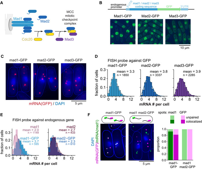
1. A

   Overview of the interactions between Mad1, Mad2, and Mad3.

2. B

   Schematic of marker‐less GFP‐tagging at the endogenous locus and representative live‐cell images of Mad1‐, Mad2‐, and Mad3‐GFP strains (average intensity projections).

3. C

   Representative images of single‐molecule mRNA FISH (smFISH) staining of S. pombe using probes against GFP (red). DNA was stained with DAPI (blue). The gamma‐value was adjusted to make the cytoplasm visible; cell shapes are outlined in blue.

4. D

   Frequency distribution of mRNA numbers per cell determined by smFISH; combined data from 3, 4, and 5 experiments, respectively, shown separately in Fig EV1C; n, number of cells. Curves show fit to a Poisson distribution.

5. E

   Frequency distribution of mRNA numbers per cell using FISH probes against the endogenous genes and using either strains expressing the GFP‐tagged gene or the endogenous, untagged gene. Curves show fit to a Poisson distribution. The difference for mad1 ⁺ is statistically significant, that for mad2 ⁺ is not (Fig EV1E). A lower mRNA number for untagged mad1 ⁺ was also observed in an independent strain.

6. F

   Co‐staining by smFISH using probes against mad1 ⁺ and GFP either in a strain expressing mad1 ⁺‐GFP as a positive control or in a strain expressing wild‐type mad1 ⁺ and mad2 ⁺‐GFP. Cytoplasmic mad1 ⁺ (green) or GFP mRNA spots (magenta) were quantified as co‐localizing or not with the respective other. For the mad1 ⁺‐GFP strain, 544 cells and a total of 1,641 mad1 spots and 1,839 GFP spots were analyzed; 48 cells were not considered as they did not contain at least one spot of each type in the cytoplasm. For the mad1 ⁺ mad2 ⁺‐GFP strain, 571 cells and a total of 1,107 mad1 spots and 1,537 GFP spots were analyzed; 158 cells were not considered since they did not contain at least one spot of each type in the cytoplasm.

Source data are available online for this figure.

Figure EV1. Additional data on Mad1, Mad2, and Mad3 tagging and mRNA numbers

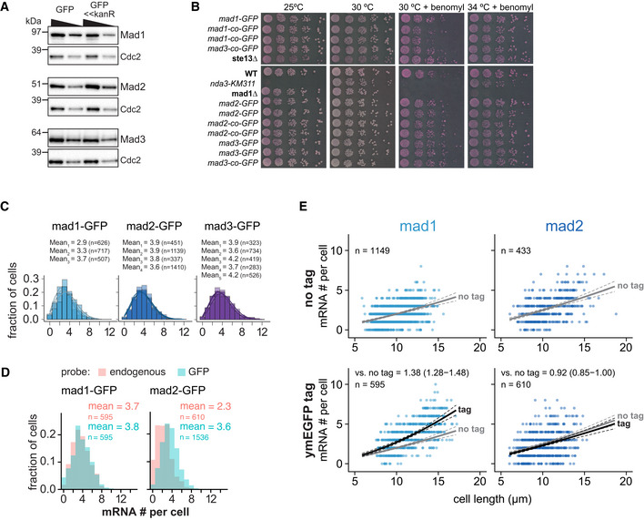
1. A

   Immunoblot comparing expression of mad1 ⁺, mad2 ⁺, and mad3 ⁺ tagged at the endogenous locus either by marker‐less insertion of yeast codon‐optimized monomeric enhanced GFP (ymEGFP, here: GFP) or conventionally with GFP‐S65T and a kanamycin‐resistance cassette (GFP<<kanR). Antibodies against the endogenous proteins were used. Cdc2 was probed as loading control. A 1:1 dilution is loaded in the second lane for each sample.

2. B

   Growth assay for the indicated strains on rich medium plates without (left side) or with benomyl (right side). The agar contains Phloxine B, which stains dead cells.

3. C

   Frequency distribution of mRNA numbers per cell. Data from individual experiments which are shown combined in Fig 1. Probes were against the GFP portion of each fusion gene. Curves show fit to a Poisson distribution.

4. D

   Frequency distribution of mRNA numbers per cell using probes against the endogenous gene or against GFP in strains expressing a GFP fusion of either mad1 ⁺ or mad2 ⁺. The comparison illustrates that for mad2 ⁺‐GFP either the endogenous probe is less sensitive, or there is considerable mRNA degradation from the 5′ end leading to fewer detected spots with a probe on the endogenous gene than on the 3′ end GFP tag.

5. E

   Same experiment as Fig 1E. Scatter plots of whole‐cell mRNA counts versus cell length. Solid lines are regression curves from generalized linear mixed model fits (gray for no tag, black for GFP‐tagged gene). Dashed lines represent 95% bootstrap confidence bands for the regression curves. Model estimates of the ratio of tagged to untagged mRNA levels with bootstrap 95% confidence intervals are included in the plots. One experiment with probes against mad1 ⁺ or mad2 ⁺ coding sequences, respectively.

Source data are available online for this figure.

Figure 2. The checkpoint genes mad1 ⁺, mad2 ⁺, and mad3 ⁺ combine short mRNA and long protein half‐lives, explaining low noise

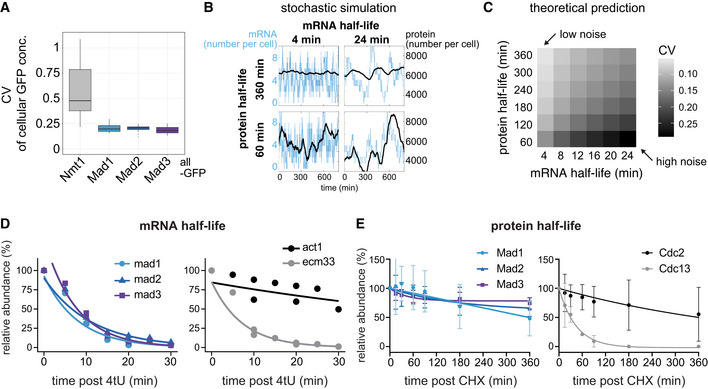
1. A

   Cellular protein noise (coefficient of variation, CV = std / mean) in live‐cell microscopy images of S. pombe; n = 7 images (Nmt1‐GFP), 11 (Mad1‐GFP), 19 (Mad2‐GFP), 10 (Mad3‐GFP); single images had 16–79 GFP‐positive and 6–94 GFP‐negative (control) cells. Boxplots show median and interquartile range (IQR); whiskers extend to values no further than 1.5 times the IQR from the first and third quartile, respectively. Mad1, Mad2, and Mad3 all showed significantly lower noise than Nmt1 (Wilcoxon rank sum test; all P < 0.001).

2. B

   Simulations of stochastic gene expression noise from selected mRNA/protein half‐life combinations assuming a constantly active promoter (see Methods). Synthesis rates were set to obtain a mean mRNA number of 4 per cell, and a mean protein number of 6,000 per cell. The x‐axis of each graph shows time, the y‐axis shows mRNA number per cell (blue) or protein number per cell (black).

3. C

   Theoretical prediction for the coefficient of variation (CV = std/mean) of the protein number per cell, assuming different mRNA and protein half‐lives, using the same underlying model as in B. Synthesis rates were adjusted to maintain a mean mRNA number per cell of 3.5, and a mean protein number per cell of 6,000 (approx. 100 nM).

4. D

   mRNA abundances by qPCR following metabolic labeling and removal of the labeled pool (two independent experiments). Lines are regression curves from generalized linear mixed model fits, excluding the measurements at t = 0 in order to accommodate for noninstantaneous labeling by 4tU. Act1⁺ and ecm33⁺ were used as long and short half‐life controls, respectively; qPCR was performed for the endogenous mRNAs. Half‐lives (95% confidence interval): mad1 ⁺ 5.6 min (4.3–8.4), mad2 ⁺ 7.7 min (6.2–10.4), mad3 ⁺ 5.2 min (4.3–6.9), act1⁺ 61.8 min (37.2–172.3), ecm33⁺ 5.0 min (4.5–5.7).

5. E

   Protein abundances after translation shut‐off with cycloheximide (CHX); n = 3 experiments, error bars = std. Lines indicate fit to a one‐phase exponential decay. Cdc2 and Cdc13 were used as long and short half‐life controls, respectively. Immunoblots for the endogenous proteins (no tag). A representative experiment shown in Appendix Fig S2E.

Source data are available online for this figure.

Figure 3. Codon‐optimization increases the steady‐state mRNA numbers of mad2 and mad3

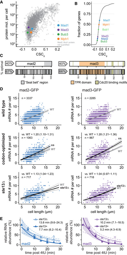
1. A

   The mean CSC value for each S. pombe gene (CSC_g) relative to protein number per cell by mass spectrometry (Carpy et al, 2014). CSC was determined using the mRNA half‐life data by Eser et al (2016) as described in Methods. Colored dots highlight proteins of interest. For Mad2 and Bub1, no protein abundance data was available.

2. B

   Cumulative frequency distribution of the CSC_g values for protein‐coding S. pombe genes. The position of spindle assembly checkpoint genes is highlighted.

3. C

   Schematic of the mad2 ⁺ and mad3 ⁺ genes. Regions coding for important structural features are highlighted. Black lines in the bottom graph indicate synonymous codon changes in the codon‐optimized version.

4. D

   Scatter plots of whole‐cell RNA counts versus cell length. Solid lines are regression curves from generalized linear mixed model fits (gray: wild type, black: codon‐optimized or ste13Δ). Dashed lines: 95% bootstrap confidence bands for the regression curves. Model estimates of the ratio relative to wild‐type mRNA are included with bootstrap 95% confidence interval in brackets. Two to five replicates per genotype.

5. E

   Time course of RNA abundances by qPCR following metabolic labeling and removal of the labeled pool (two independent experiments). Solid lines: regression curves from generalized linear mixed model fits (dark = ste13 ⁺, light = ste13Δ), excluding t = 0 to accommodate for non‐instantaneous labeling by 4tU. Shaded area: 95% bootstrap confidence band for ste13 ⁺; dashed lines: 95% bootstrap confidence band for ste13Δ. Half‐life estimates are included with 95% bootstrap confidence intervals in brackets. See Fig EV2C for additional statistics. The ste13 ⁺ data are the same as in Fig 2.

Source data are available online for this figure.

Figure EV2. Additional data on mad2 ⁺ and mad3 ⁺ mRNA numbers and half‐lives after codon‐optimization or ste13 ⁺ deletion

1. A

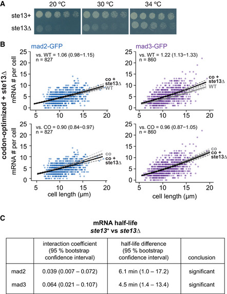
   Growth assay for wild‐type and ste13Δ cells on minimal medium plates.

2. B

   Scatter plots of whole‐cell mRNA counts versus cell length for cells expressing codon‐optimized mad2‐ or mad3‐GFP and deleted for ste13 ⁺. Solid lines are regression curves from generalized linear mixed model fits; black for the genotype shown, gray for the respective reference: wild type (WT) in the first row, codon‐optimized (co) in the second row. Dashed lines represent 95% bootstrap confidence bands for the regression curves. Model estimates of the mRNA level relative to the reference with bootstrap 95% confidence intervals in parentheses are included in the plots. Control curves for upper panels from wild‐type mad2 ⁺ and mad3 ⁺ data in Fig 3D, and for lower panels from codon‐optimized mad2 and mad3 data in Fig 3D. Two to five replicates per genotype.

3. C

   Statistical significance for mRNA half‐life changes after deletion of ste13 ⁺. First and second columns show estimates and 95% bootstrap confidence intervals for the model interaction coefficient and the half‐life difference, respectively. The change in half‐life after deletion of ste13 ⁺ was considered significant if the 95% bootstrap confidence intervals for the interaction coefficient and the half‐life difference excluded 0.

Source data are available online for this figure.

Figure EV3. Cytoplasmic and nuclear FISH data for mad2 ⁺ and mad3 ⁺

Scatter plots of cytoplasmic and nuclear mRNA counts versus cell length for mad2 ⁺ and mad3 ⁺. Solid lines are regression curves from generalized linear mixed model fits; gray is wild type (WT) in rows 1–4 and codon‐optimized (co) in row 5, black is the genotype indicated. Dashed lines represent 95% bootstrap confidence bands for the regression curves. Model estimates for the mRNA ratio between the genotype indicated on the left and the respective reference are included in the plots with bootstrap 95% confidence intervals in parentheses. Same experiments as whole‐cell data in Figs 1D and 3D, and EV2B. Two to five replicates per genotype. Source data are available online for this figure.

Figure 4. Codon‐optimization increases the protein concentrations of Mad2 and Mad3

1. A

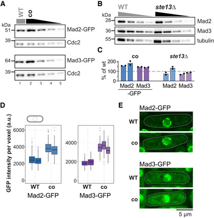
   Immunoblot of S. pombe protein extracts from cells expressing wild‐type (WT) or codon‐optimized (co) Mad2‐GFP or Mad3‐GFP probed with antibodies against GFP and Cdc2 (loading control). Lanes 3–5 are a 1:1 dilution series of the extract from cells expressing the codon‐optimized version.

2. B

   Immunoblot of protein extracts from wild‐type (WT) or ste13Δ strains probed with antibodies against Mad2, Mad3, and tubulin (loading control). A 1:1 dilution series was loaded for quantification.

3. C

   Estimates of the protein concentration relative to wild‐type conditions from experiments such as in (A) and (B). Bars are experimental replicates, dots are technical replicates. Two‐sided t‐tests: P = 0.03 (Mad2‐co), 0.004 (Mad3‐co), 0.82 (Mad2 ste13Δ), 0.15 (Mad3 ste13Δ).

4. D

   Whole‐cell GFP concentration from individual live‐cell fluorescence microscopy experiments (a.u., arbitrary units). Boxes show median and interquartile range (IQR); whiskers extend to values no further than 1.5 times the IQR from the first and third quartile, respectively. Codon‐optimized concentration significantly higher than wild type for both genes (generalized linear mixed model). Mad2‐GFP: n = 468 and 413; Mad2‐co‐GFP: n = 206 and 366; Mad3‐GFP: n = 224 and 127; Mad3‐co‐GFP: n = 160, 450 and 212 cells.

5. E

   Representative images from one of the experiments in (D). A single Z‐slice is shown. Cells are outlined in gray.

Source data are available online for this figure.

Figure 5. Codon‐optimization and ste13 ⁺ deletion do not significantly affect the steady‐state mRNA number of mad1 ⁺

1. A

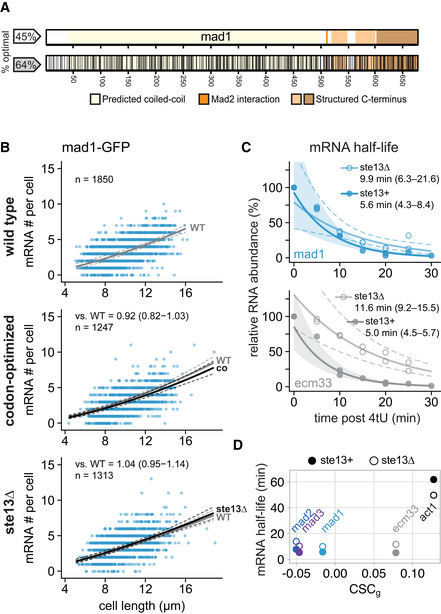
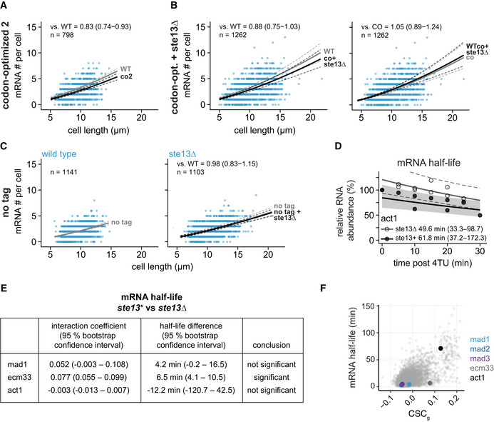
   Schematic of the mad1 ⁺ gene. Regions coding for important structural features are highlighted. Black lines in the bottom graph indicate synonymous codon changes in the codon‐optimized version.

2. B

   Scatter plots of whole‐cell mRNA counts versus cell length. Solid lines are regression curves from generalized linear mixed model fits (gray: wild type, black: codon‐optimized or ste13Δ). Dashed lines: 95% bootstrap confidence bands for the regression curves. Model estimates of the ratio relative to wild‐type mRNA are included with bootstrap 95% confidence interval in brackets. Two to three replicates per genotype.

3. C

   Time course of RNA abundances by qPCR following metabolic labeling and removal of the labeled pool (two independent experiments). Solid lines: regression curves from generalized linear mixed model fits (dark = ste13 ⁺, light = ste13Δ), excluding t = 0 to accommodate for non‐instantaneous labeling by 4tU. Shaded area: 95% bootstrap confidence band for ste13 ⁺; dashed lines: 95% bootstrap confidence band for ste13Δ. Half‐life estimates are included with 95% bootstrap confidence intervals in brackets. See Fig EV4E for additional statistics. The ste13 ⁺ data are the same as in Fig 2.

4. D

   Comparison between mean CSC values for selected genes (CSC_g) and mRNA half‐life measured with or without deletion of ste13 ⁺. mRNA half‐life estimates from Figs 3E and 5C, and EV4D.

Source data are available online for this figure.

Figure EV4. Additional data on mad1 ⁺ mRNA number and half‐life after codon‐optimization or ste13 ⁺ deletion

1. A

   Scatter plot of whole‐cell mRNA counts versus cell length. Solid lines are regression curves from generalized linear mixed model (GLMM) fits; black for the genotype shown (co2), gray for the wild‐type (WT) reference. Dashed lines represent 95% bootstrap confidence bands for the regression curves. Model estimates for the mRNA ratio between the genotypes indicated are included in the plots with bootstrap 95% confidence intervals in parentheses. Two to three replicates per genotype.

2. B

   As in (A). Black regression line for the genotype shown (co + ste13Δ), gray for the respective reference, wild type (WT) or codon‐optimized (co). Two to three replicates per genotype.

3. C

   Scatter plots for whole‐cell mRNA counts of untagged mad1 ⁺ in ste13 ⁺ (left) or ste13Δ (right) cells, similar to (A). The regression curve for untagged mad1 ⁺ in ste13 ⁺ is shown in gray, that for untagged mad1 ⁺ in ste13Δ in black. Probes were against the mad1 ⁺ coding sequence. One to three replicates per genotype.

4. D

   Time course of RNA abundances by qPCR following metabolic labeling and removal of the labeled pool (two independent experiments). Solid lines are regression curves from GLMM fits (black = ste13 ⁺, gray = ste13Δ), excluding the measurements at t = 0 to accommodate for noninstantaneous labeling by 4tU. Shaded area is 95% bootstrap confidence band for the ste13 ⁺ curve and dashed lines indicate 95% bootstrap confidence band for the ste13Δ curve. Half‐life estimates with 95% bootstrap confidence intervals are included on the plot. The ste13 ⁺ data are the same as in Fig 2.

5. E

   Statistical significance for mRNA half‐life changes after deletion of ste13 ⁺. First and second columns show estimates and 95% bootstrap confidence intervals for the model interaction coefficient and the half‐life difference, respectively. The change in half‐life after deletion of ste13 ⁺ was considered significant if the 95% bootstrap confidence intervals for the interaction coefficient and the half‐life difference excluded 0.

6. F

   CSC_g values (this study) and mRNA half‐lives (from Eser et al, 2016) for protein‐coding S. pombe genes with the indicated genes highlighted.

Source data are available online for this figure.

Figure EV5. Cytoplasmic and nuclear FISH data for mad1 ⁺

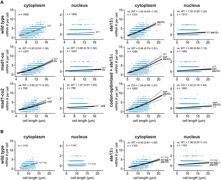
1. A

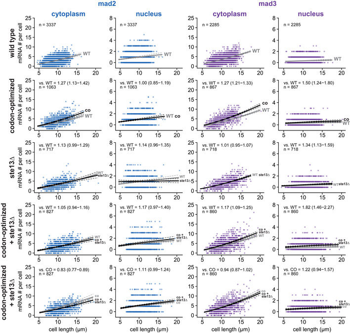
   Scatter plots of cytoplasmic and nuclear mRNA counts versus cell length for mad1 ⁺. Solid lines are regression curves from generalized linear mixed model fits; gray is wild‐type (WT) mad1 ⁺‐GFP for all panels, except the bottom row on the right side, where it is codon‐optimized mad1‐GFP (co), black is the genotype indicated on the left. Dashed lines represent 95% bootstrap confidence bands for the regression curves. Model estimates for the mRNA ratio between the genotype indicated on the left and the respective reference are included in the plots with bootstrap 95% confidence intervals in parentheses. Same experiments as whole‐cell data in Figs 1D and 5B, and EV4A and B. Two to three replicates per genotype.

2. B

   Similar to (A) but for untagged mad1 ⁺. Solid lines are regression curves from generalized linear mixed model fits; gray is untagged wild‐type mad1 ⁺ for all panels, black is untagged mad1 ⁺ in ste13Δ. One to three replicates per genotype. Same experiments as whole‐cell data in Fig EV4B.

Source data are available online for this figure.

Figure 6. Codon identity in mad1 ⁺ is important for proper protein concentration

1. A

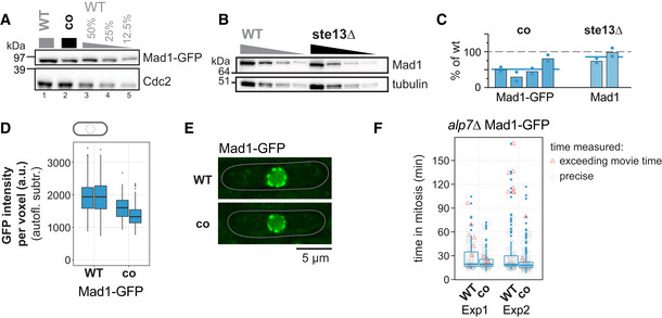
   Immunoblot of S. pombe protein extracts from cells expressing wild‐type (WT) or codon‐optimized (co) Mad1‐GFP probed with antibodies against GFP and Cdc2 (loading control). Lanes 3–5 are a dilution series of the extract from wild‐type cells.

2. B

   Immunoblot of protein extracts from wild‐type (WT) or ste13Δ strains probed with antibodies against Mad1 and tubulin (loading control). A 1:1 dilution series was loaded for quantification. Tubulin blot is the same as in Fig 4B.

3. C

   Estimates of the protein concentration relative to wild‐type conditions from experiments such as in (A) and (B). Bars are experimental replicates, dots are technical replicates. Blue lines indicate the mean of all experiments. Two‐sided t‐tests: P = 0.005 (Mad1‐co, n = 4 experimental replicates); P = 0.16 (Mad1 ste13Δ, n = 2).

4. D

   Whole‐cell GFP concentration from individual live‐cell fluorescence microscopy experiments (a.u. = arbitrary units). Boxplots show median and interquartile range (IQR); whiskers extend to values no further than 1.5 times the IQR from the first and third quartile, respectively. Codon‐optimized concentration significantly lower than wild type (generalized linear mixed model). Mad1‐GFP: n = 197 and 224; Mad1‐co‐GFP: n = 80 and 377 cells.

5. E

   Representative images from one of the experiments in (D). An average projection of three Z‐slices is shown; cells are outlined in gray.

6. F

   Live‐cell imaging for time spent in mitosis. The alp7 ⁺ gene was deleted to increase the likelihood of spindle assembly checkpoint activation. Localization of Plo1‐tdTomato to spindle‐pole bodies was used to judge entry into and exit from mitosis (also see Appendix Fig S4). Exp1: n = 73 (WT) and 94 cells (co); Exp2: n = 126 (WT) and 152 cells (co). Boxplots show median and interquartile range (IQR); whiskers extend to values no further than 1.5 times the IQR from the first and third quartile, respectively. Measurements for individual cells are shown in addition (gray circles if measurement was exact, red triangles if end of mitosis was not captured because imaging ended). Difference between WT and co: P = 0.14 (Exp1) and 0.15 (Exp2) by Kolmogorov–Smirnov test.

Source data are available online for this figure.

Figure 7. Mad1 homodimers assemble co‐translationally

1. A

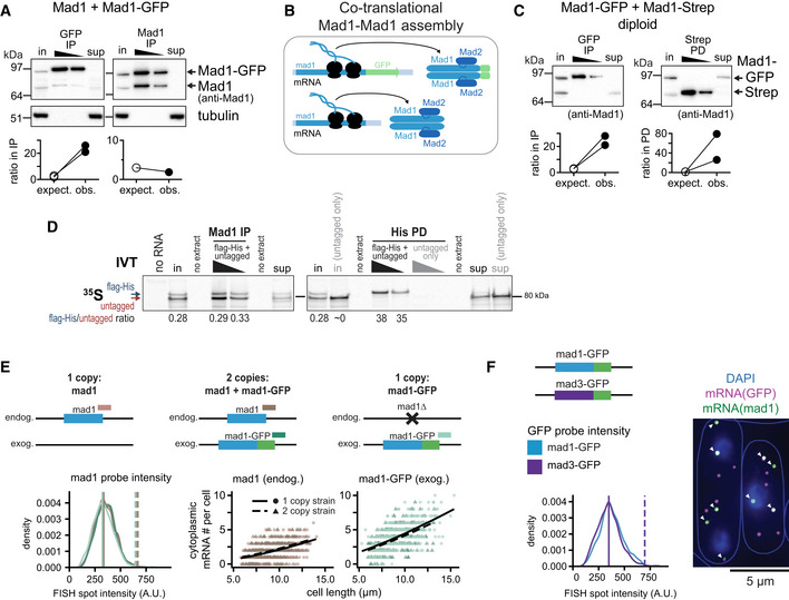
   Top: Immunoprecipitation (IP) with anti‐GFP or anti‐Mad1 from extracts of haploid S. pombe cells expressing both untagged and GFP‐tagged Mad1, probed with antibodies against Mad1 and tubulin; in = input (2.5% of extract for IP), sup = supernatant after IP. Bottom: Comparison between the observed (obs.) and the expected (expect.) ratio between Mad1‐GFP and untagged Mad1 in the IP given their ratio in the input (see Fig EV6A); two and one experiment(s), respectively. One more GFP‐IP from the same strain was unquantifiable, because no second band was visible in the IP.

2. B

   Schematic illustrating that Mad1‐Mad1 complex assembly likely takes place co‐translationally with only proteins synthesized from the same mRNA being combined.

3. C

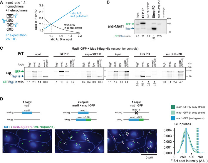
   Top: Anti‐GFP immunoprecipitation (IP) and Strep pull‐down (PD) from extracts of diploid cells expressing Mad1‐GFP and Mad1‐Strep from the two endogenous loci; membrane probed with anti‐Mad1; in, input (7% of extract for IP/PD), sup, supernatant after IP/PD. Bottom: as in (A), 2 experiments each. See Fig EV6 for a quantified experiment. The experiment shown at the top and two more GFP‐IPs from the same strain were unquantifiable, because no second band was visible in the IP.

4. D

   In vitro translation (IVT) of Mad1‐flag‐His and untagged Mad1 in the presence of ³⁵S‐labeled Methionine and Cysteine, followed by Mad1 immunoprecipitation (IP) or His pull‐down (PD); in, input (9.5% of extract for IP/PD), sup, supernatant after IP/PD. An IVT with only untagged Mad1 was used to check for specificity of the His PD (right side). Shown is the autoradiograph after SDS‐PAGE with quantification of the Mad1‐flag‐His to untagged Mad1 ratio in select lanes.

5. E

   Test for mRNA dimerization by single‐molecule mRNA FISH; probes against mad1 ⁺ and GFP. Top: Schematic of genotypes. Example pictures in Fig EV6. Bottom left: Intensity of cytoplasmic mad1 ⁺ mRNA spots in the different strains. For the 2 copy strain, a mad1 ⁺ spot was classified as mad1 ⁺‐GFP if it was co‐localizing with a GFP spot, and as mad1 ⁺ otherwise. Colors as indicated in the schematic. Vertical solid line: peak of each density plot; dashed line: theoretical position of a double‐intensity peak. Number of spots analyzed: mad1 ⁺ (1 copy strain) = 921, mad1 ⁺ (2 copy strain) = 637, mad1 ⁺‐GFP (2 copy strain) = 982, mad1 ⁺‐GFP (1 copy strain) = 1,699. Bottom right: Counts of cytoplasmic mad1 ⁺ or mad1 ⁺‐GFP mRNA from the same experiment with generalized linear mixed model fits as lines. Number of cells: 1 copy strain mad1 ⁺ = 478, 2 copy strain = 327, 1 copy strain mad1 ⁺‐GFP = 466.

6. F

   Experiment similar to (E), except that cells expressing both mad1 ⁺‐GFP and mad3 ⁺‐GFP from the respective endogenous locus were probed with FISH probes against mad1 ⁺ and GFP mRNA. A GFP spot was classified as mad1 ⁺‐GFP if it was co‐localizing with a mad1 ⁺ spot (arrowheads), and as mad3 ⁺‐GFP otherwise. The intensity of GFP spots was quantified. Vertical solid line: peak of each density plot; dashed line: theoretical position of a double‐intensity peak. Number of spots analyzed: mad1 ⁺‐GFP = 987, mad3 ⁺‐GFP = 1,299.

Source data are available online for this figure.

Figure EV6. Additional experiments supporting that Mad1 homodimers assemble co‐translationally

1. A

   Theoretical considerations: if, for two different copies of Mad1, homodimer and heterodimer formation was equally likely, and the ratio in the input was 1:1, one would expect a ratio of 2:1 in the pull‐down. Expectations for other input ratios are shown in the graph. For typical input ratios in our experiments, the maximum expected ratio in IP/PD is around 4:1, whereas we typically observe 10:1 or higher.

2. B

   Replicate experiment for Fig 7C; one of the experiments quantified at the bottom of Fig 7C. Anti‐GFP immunoprecipitation (IP) and Strep pull‐down (PD) from extracts of diploid cells expressing Mad1‐GFP and Mad1‐Strep from the two endogenous loci; membrane probed with anti‐Mad1; input is 3% of extract used for IP/PD, sup = supernatant. Numbers at the bottom show the quantification of the Mad1‐GFP to Mad1‐Strep ratio. The last lane contains extract of a diploid strain with both copies of endogenous mad1 ⁺ deleted.

3. C

   In vitro translation (IVT) of Mad1‐GFP and Mad1‐flag‐His in the presence of ³⁵S‐labeled Methionine and Cysteine, followed by GFP immunoprecipitation (IP) or His pull‐down (PD); input is 10% of extract used for IP/PD, sup = supernatant. IVTs with only Mad1‐flag‐His, or only Mad1‐GFP were used to control for the specificity of the IP/PD. High RNA conc. is 40 ng/μl mad1‐GFP and 35 ng/μl mad1‐flag‐His; the medium and low concentrations are 1:10 and 1:100 dilutions of the “high” mix. Shown is the autoradiograph after SDS‐PAGE with quantification of the Mad1‐GFP to Mad1‐flag‐His ratio. One out of two experiments with similar results.

4. D

   Same experiment as in Fig 7E. Representative images from each strain with co‐localizing mad1 ⁺ and GFP spots marked by arrowheads. Right side: Intensity of cytoplasmic GFP mRNA spots in the different strains. Vertical solid line: peak of each density plot; dashed line: theoretical position of a double‐intensity peak. Number of spots analyzed: mad1 ⁺‐GFP (2 copy strain) = 1,178, mad1 ⁺‐GFP (1 copy strain) = 1,796, mad1 ⁺‐GFP expressed from the endogenous locus (not shown schematically on the left) = 987.

Source data are available online for this figure.

References

-
- Aravind L, Koonin EV (1998) The HORMA domain: A common structural denominator in mitotic checkpoints, chromosome synapsis and DNA repair. Trends Biochem Sci 23: 284–286 - PubMed
- Arganda‐Carreras I, Kaynig V, Rueden C, Eliceiri KW, Schindelin J, Cardona A, Sebastian Seung H (2017) Trainable Weka segmentation: a machine learning tool for microscopy pixel classification. Bioinformatics 33: 2424–2426 - PubMed
- Bähler J, Wu JQ, Longtine MS, Shah NG, McKenzie A 3rd, Steever AB, Wach A, Philippsen P, Pringle JR (1998) Heterologous modules for efficient and versatile PCR‐based gene targeting in Schizosaccharomyces pombe . Yeast 14: 943–951 - PubMed
Publication types
MeSH terms
Substances
Grants and funding
LinkOut - more resources
Full Text Sources
Molecular Biology Databases