An atlas of endogenous DNA double-strand breaks arising during human neural cell fate determination

Abstract

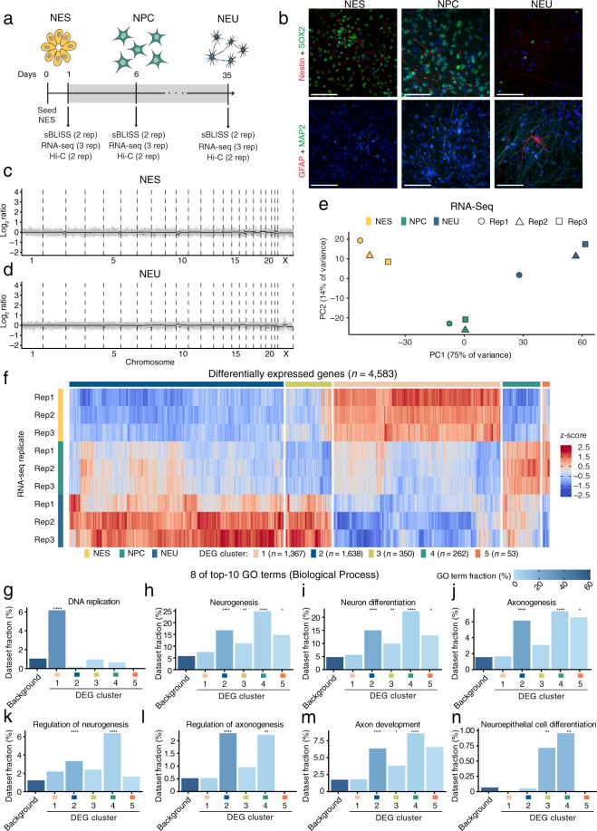
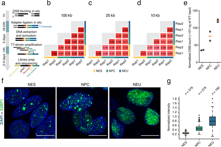
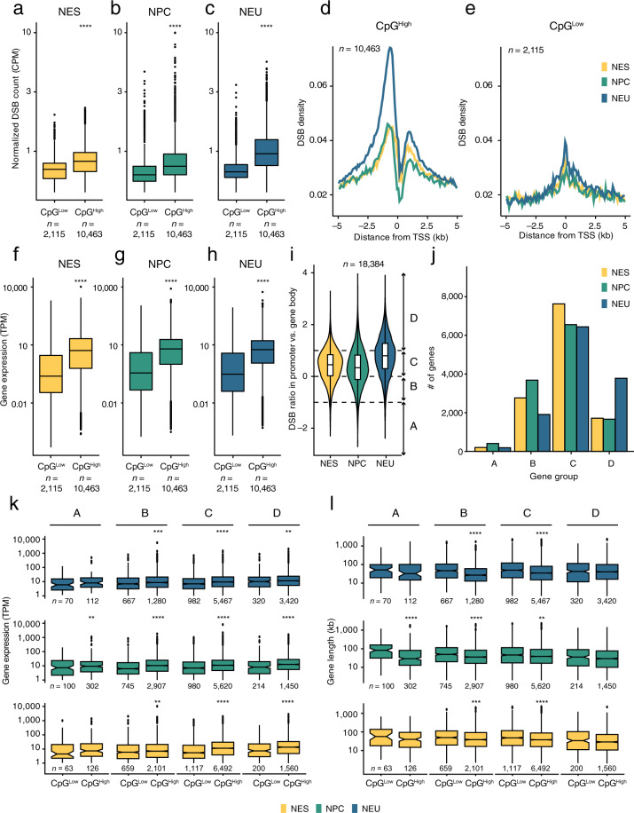
Endogenous DNA double-strand breaks (DSBs) occurring in neural cells have been implicated in the pathogenesis of neurodevelopmental disorders (NDDs). Currently, a genomic map of endogenous DSBs arising during human neurogenesis is missing. Here, we applied in-suspension Breaks Labeling In Situ and Sequencing (sBLISS), RNA-Seq, and Hi-C to chart the genomic landscape of DSBs and relate it to gene expression and genome architecture in 2D cultures of human neuroepithelial stem cells (NES), neural progenitor cells (NPC), and post-mitotic neural cells (NEU). Endogenous DSBs were enriched at the promoter and along the gene body of transcriptionally active genes, at the borders of topologically associating domains (TADs), and around chromatin loop anchors. NDD risk genes harbored significantly more DSBs in comparison to other protein-coding genes, especially in NEU cells. We provide sBLISS, RNA-Seq, and Hi-C datasets for each differentiation stage, and all the scripts needed to reproduce our analyses. Our datasets and tools represent a unique resource that can be harnessed to investigate the role of genome fragility in the pathogenesis of NDDs.

Fig. 1

Validation of the model system of human neurogenesis used in this study. (a) Timeline of 2D culture of neuroepithelial stem (NES) cell differentiation to neural progenitor cells (NPC) and neuronal (NEU) cells. The rose rectangle indicates the period during which the cells were kept in differentiation conditioning medium (see Methods). Cells were harvested at three timepoints and processed for sBLISS, RNA-Seq, and Hi-C (see Supplementary Table 1 for the list of datasets). Note that different batches of NES cells from different passages (max 5 passages apart) were used for performing multiple replicate (rep) experiments with each technique. (b) Maximum z-projections of wide-field epifluorescence microscopy z-stacks showing the expression of different markers of neuronal lineage at the same days (D) of differentiation shown in (a). Scale bars, 100 μm. (c,d) Genome-wide DNA copy number profiles (100 kb resolution) of NES and NEU cells. Each grey dot represents one 100 kb genomic bin. The black lines indicate the median Log2 ratio between the observed and expected read counts per bin along each chromosome. (e) Principal component analysis of the RNA-Seq datasets (Datasets 7–15, see Supplementary Table 1). PC, principal component. Rep, replicate. (f) Hierarchical clustering of differentially expressed genes (DEG) between NES, NPC, and NEU cells. Rep, replicate. (g–n) Enrichment of 8 of the top-10 gene ontology (GO) terms associated with the differentially expressed genes shown in (f), in each of the five clusters shown in (f) or in the remaining protein-coding genes (Background).

Fig. 2

Overview and validation of sBLISS. (a) sBLISS workflow and schematic representation of the adapters used to tag individual DSB ends and to amplify the genomic DNA (gDNA) sequence downstream by in vitro transcription. UMI, unique molecular identifier. T7, T7 phage RNA polymerase. RA3/5, Illumina adapters. (b–d) Reproducibility of DSB counts at different genomic resolutions between two sBLISS replicate (Rep) experiments in NES, NPC, and NEU cells. The numbers in the red squares represent the Pearson’s correlation coefficient. (e) Normalized counts of DSB ends detected by sBLISS in each of the six sBLISS datasets described here. The DSB counts were normalized to the amount (in ng) of genomic DNA used as input in the in vitro transcription (IVT) step in sBLISS. Each grey dot represents one replicate experiment. Orange bars, mean value. (f) Maximum z-projections of wide-field epifluorescence microscopy z-stacks showing the expression of the DSB marker 53BP1 in NES, NPC, and NEU cells. Representative fields of view are shown. Scale bars, 50 μm. Blue, DNA staining with Hoechst 33342. (g) Normalized 53BP1 nuclear intensity in the images of which those shown in (f) are representative examples. For each segmented nucleus, we normalized the intensity in the fluorescence channel of the 53BP1 antibody to the intensity of the DNA staining channel (see Methods). Each boxplot extends from the 25th to the 75th percentile, the horizontal bars represent the median, and whiskers extend from –1.5 × IQR to + 1.5 × IQR from the closest quartile, where IQR is the inter-quartile range. Black dots, outliers.

Fig. 3

Endogenous DSBs are enriched in the promoter region and along the gene body of highly expressed protein-coding genes. (a–c) Distributions of normalized DSB counts in a 3 kb window (from 2 kb upstream to 1 kb downstream) around the transcription start sites (TSS) of human protein-coding genes classified in four different quartiles (Q) based on their expression levels determined by RNA-Seq. CPM, DSB count per million reads calculated as number of DSBs divided by number of reads times one million. n, number of genes in each expression quartile. Asterisks indicate a P value lower than 0.0001 (Wilcoxon test, two-tailed) comparing the distribution below them with the Q1 distribution in the same plot. (d–f) Same as in (a–c), but for DSBs along the gene body of human protein-coding genes (from the first TSS to the last transcription end site of each gene). The part of the boxplots highlighted in grey is magnified on the right. (g,h) Visualization of mapped DSBs along two genes using the squish option in the UCSC genome browser. The dashed red rectangles indicate the enrichment of DSBs around the TSSs of the two genes. In all the boxplots shown in the figure, each boxplot extends from the 25th to the 75th percentile, the horizontal bar represents the median, and whiskers extend from –1.5 × IQR to + 1.5 × IQR from the closest quartile, where IQR is the inter-quartile range. Black dots, outliers.

Fig. 4

CpG-rich promoters are highly fragile. (a–c) Distributions of normalized DSB counts in a 3 kb window (from 2 kb upstream to 1 kb downstream) around the transcription start sites (TSS) of human protein-coding genes, for genes with high (CpG^High) or low (CpG^Low) levels of CpG dinucleotides in their promoter region. CPM, DSB count per million reads calculated as number of DSBs divided by number of reads times one million. n, number of genes in each group. (d,e) Metaprofiles of the DSB density around the TSS of human protein-coding genes classified as CpG^High (d) or CpG^Low (e) based on the frequency of CpG dinucleotides in their promoter region. n, number of genes. (f–h) Same as in (a–c) but for gene expression levels. TPM, transcripts per million. (i) Distributions of the ratio between the number of DSBs in the promoter (from 2 kb upstream to 1 kb downstream of the TSS) and along the gene body (from the first TSS of the gene to the last transcription end site), for all human protein-coding genes (n) in NES, NPC, and NEU cells. Each distribution was arbitrarily divided into four regions as following: A (–Inf; –1]; B (–1; 0]; C (0; 1]; D (1; Inf]. The violin plots extend from minimum to maximum, and the boxplots inside the violins extend from the 25th to the 75th percentile, with the horizontal bar representing the median, and whiskers extending from –1.5 × IQR to + 1.5 × IQR from the closest quartile, where IQR is the inter-quartile range. (j) Number of genes in each of the four groups shown in (i). (k) Distributions of gene expression levels measured by RNA-Seq in the four gene groups shown in (i), for genes classified as CpG^High or CpG^Low based on the frequency of CpG dinucleotides in their promoter region. The number of genes (n) in each group is shown below each boxplot. (l) Same as in (k) but for gene length in kiloSbases (kb). Gene length was calculated as the distance from the TSS to the transcription end site of each gene. In all the boxplots shown in the figure, each boxplot extends from the 25th to the 75th percentile, the horizontal bar represents the median, and whiskers extend from –1.5 × IQR to + 1.5 × IQR from the closest quartile, where IQR is the inter-quartile range. Black dots, outliers. The asterisks in (a–c), (f–h) and (k,m) indicate a P value less than 0.01 (**), 0.001 (***) or 0.0001 (****) (Wilcoxon test, two-tailed). ns, not significant.

Fig. 5

Endogenous DSBs are enriched in the active (A) chromatin compartment. (a) Concordance matrix revealing high similarity between the Hi-C replicates generated from NES, NPC, and NEU cells (100 kb resolution). (b) Fraction of the genome (1 Mb resolution) belonging to the A compartment as determined by Hi-C. (c) Fraction of 1 Mb genomic regions that either belong to the same (A → A and B → B) or switching compartment (A → B or B → A) during the transition from NES to NPC. (d) Same as in (c) but for the transition from NPC to NEU. (e–g) Distributions of normalized DSB counts in 1 Mb genomic regions belonging to the A or B compartment in NES (a), NPC (b), and NEU (c) cells. CPM, DSB count per million reads calculated as number of DSBs divided by number of reads times one million. n, number of 1 Mb genomic regions in each compartment. Asterisks: P value less than 0.0001 (Wilcoxon test, two-tailed). (h–j) Same as in (e–g) but comparing genomic regions that do not change (Stable) or that switch (Changing) compartment type during the transition from NES to NEU. (k–m) Same as in (h–j) but distinguishing between A/B compartments. In all the violin plots in (e–m), the violins extend from minimum to maximum and the boxplots inside each violin extend from the 25th to the 75th percentile. The horizontal bars represent the median and whiskers extend from –1.5 × IQR to + 1.5 × IQR from the closest quartile, where IQR is the inter-quartile range. The asterisks in (e–m) indicate a P value less than 0.01 (**), 0.001 (***) or 0.0001 (****) (Wilcoxon test, two-tailed). ns, not significant.

Fig. 6

Endogenous DSBs are enriched at TAD boundaries and around chromatin loop anchors. (a) Distributions of the sizes of TADs identified from Hi-C datasets in NES, NPC, and NEU cells. n, number of TADs. P values are indicated above the violin plots. The violin plots extend from minimum to maximum, and the boxplots inside the violins extend from the 25th to the 75th percentile, with the horizontal bar representing the median, and whiskers extending from –1.5 × IQR to + 1.5 × IQR from the closest quartile, where IQR is the inter-quartile range. The asterisks indicate a P value less than 0.0001 (Wilcoxon test, two-tailed). ns, not significant. (b) Metaprofile of the average insulation score of TAD boundaries for each of the three differentiation stages. See Methods for how the average insulation score was calculated from the Hi-C datasets. (c,d) Fraction of TADs spanning genomic regions (1 Mb resolution) belonging to the same (c) or to a different (d) compartment type. (e) Metaprofile of the DSB density around TAD boundaries identified in NES, NPC, and NEU cells based on Hi-C data. n, number of TADs. (f,g) Metaprofiles of DSB enrichment around the upstream (f) and downstream (g) anchor site of chromatin loops identified by Hi-C in NES, NPC, and NEU cells. n, number of loops. (h) Same as in (f,g) but for DSB enrichment around CTCF factor binding motifs. n, number of CTCF motifs. (i) Fraction of TADs belonging to one of six categories: (1) Early Appearing (EA); (2) Early Disappearing (ED); (3) Late Appearing (LA); (4) Late Disappearing (LD); (5) Dynamic (D); and (6) Highly Common (HC), based on whether and when TADs disappear or appear during the differentiation of NES cells to NEU. See Methods for how the classification was performed. (j) Same as in (i) but separately for each chromosome. (k) Same as in (i) but for chromatin loops. Note that the last category (grey) is now referred to as Conserved Loop (CL). (l–n) Distributions of the DSB burden per kb in a genomic region of 50 kb around each TAD boundary in NES (l), NPC (m), and NEU (n) cells. Categories assigned as in (i). (o–q) Same as in (l–n) but for chromatin loops. In all the boxplots in (l–q), each boxplot extends from the 25th to the 75th percentile, the horizontal bars represent the median, and whiskers extend from –1.5 × IQR to + 1.5 × IQR from the closest quartile, where IQR is the inter-quartile range. Black dots, outliers.

Fig. 7

Endogenous DBSs are enriched at the promoter and along the gene body of genes associated with increased risk for schizophrenia (SCZ) and autism spectrum disorder (ASD). (a–c) Distributions of normalized DSB counts in the promoter region (from 2 kb upstream to 1 kb downstream) around the transcription start sites (TSS) of genes associated with SCZ risk (see Supplementary Data in ref. ) or background genes comprising all human protein-coding genes except the examined SCZ risk genes. CPM, DSB count per million reads calculated as number of DSBs divided by number of reads times one million. n, number of genes in each group. (d–f) Same as in (a–c) but for normalized DSB counts along the gene body (from the first TSS of the gene to the last transcription end site). (g–i) Same as in (a–c) but for genes associated with ASD risk (see Table S2 in ref. ). (j–l) Same as in (h–j) but for normalized DSB counts along the gene body. The asterisks in (a–l) indicate a P value less than 0.01 (**), 0.001 (***) or 0.0001 (****) (Wilcoxon test, two-tailed).

Fig. 8

Top-fragile genes associated with increased risk for schizophrenia (SCZ) and autism spectrum disorder (ASD). (a) Normalized DSB counts in the promoter region (from 2 kb upstream to 1 kb downstream of the transcription start site (TSS)) for the ten most fragile genes associated with SCZ risk in NES, NPC, and NEU cells. CPKM, DSB count per kilobase per million reads calculated as number of DSBs divided by number of reads times one million divided by gene width times 1,000. (b) Same as in (a) but for the ten most fragile genes associated with ASD risk. (c,d) Visualization of mapped DSBs along two of the top-fragile genes shown in (a) and (b) using the squish option in the UCSC genome browser. The dashed red rectangles indicate the enrichment of DSBs around the TSS of the two genes. (e) Distributions of gene expression levels in SCZ risk genes and background genes (all human protein-coding genes except SCZ risk genes) in NES, NPC, and NEU cells. Asterisks indicate a P value less than 0.0001 (Wilcoxon test, two-tailed). TPM, transcripts per million. (f) Same as in (e) but for ASD risk genes.

References

1. Scully R, Panday A, Elango R, Willis NA. DNA double-strand break repair-pathway choice in somatic mammalian cells. Nat. Rev. Mol. Cell Biol. 2019;20:698–714. - PMC - PubMed
1. Tubbs A, Nussenzweig A. Endogenous DNA Damage as a Source of Genomic Instability in Cancer. Cell. 2017;168:644–656. - PMC - PubMed
1. Bouwman, B. A. M. & Crosetto, N. Endogenous DNA Double-Strand Breaks during DNA Transactions: Emerging Insights and Methods for Genome-Wide Profiling. Genes9 (2018). - PMC - PubMed
1. Gothe HJ, et al. Spatial Chromosome Folding and Active Transcription Drive DNA Fragility and Formation of Oncogenic MLL Translocations. Mol. Cell. 2019;75:267–283.e12. - PubMed
1. Canela A, et al. Topoisomerase II-Induced Chromosome Breakage and Translocation Is Determined by Chromosome Architecture and Transcriptional Activity. Mol. Cell. 2019;75:252–266.e8. - PMC - PubMed
Publication types