Mathematical relationships between spinal motoneuron properties

Abstract

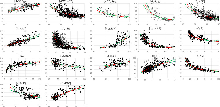
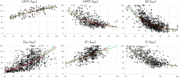
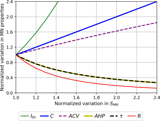
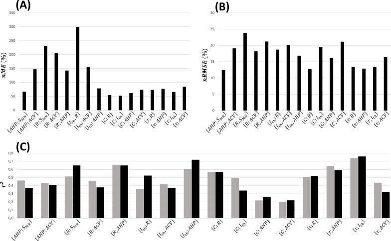
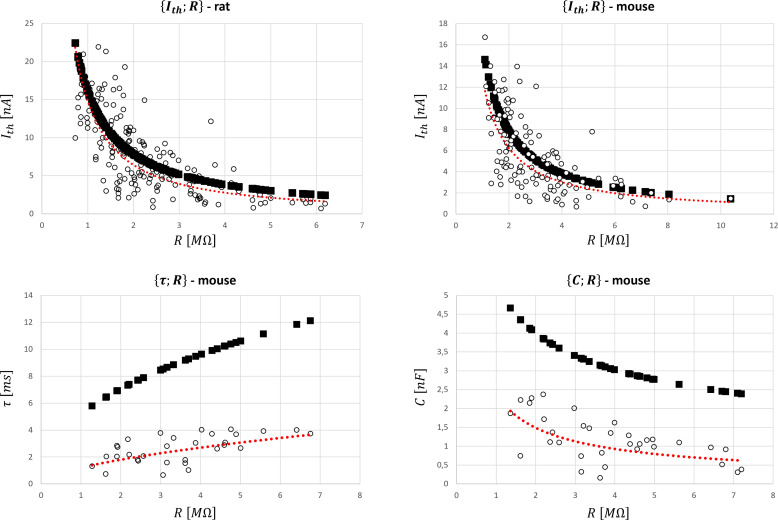
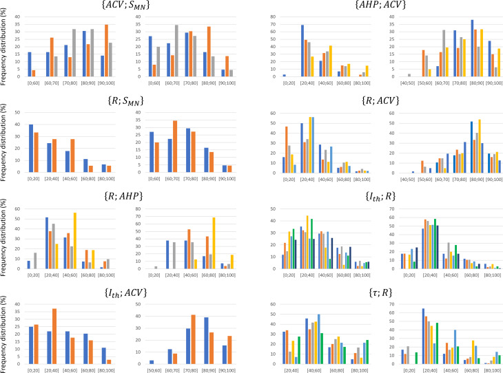
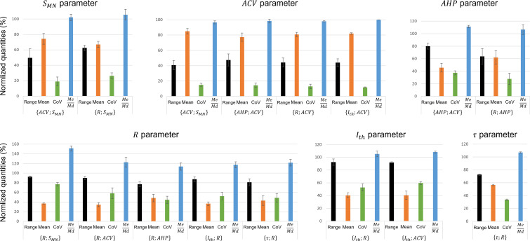
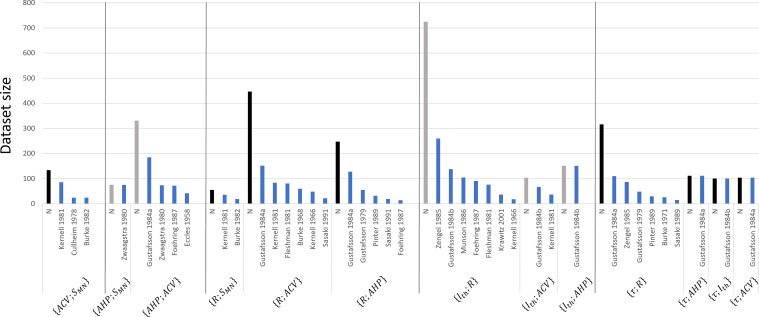
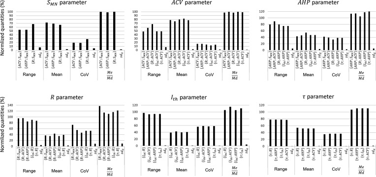
Our understanding of the behaviour of spinal alpha-motoneurons (MNs) in mammals partly relies on our knowledge of the relationships between MN membrane properties, such as MN size, resistance, rheobase, capacitance, time constant, axonal conduction velocity, and afterhyperpolarization duration. We reprocessed the data from 40 experimental studies in adult cat, rat, and mouse MN preparations to empirically derive a set of quantitative mathematical relationships between these MN electrophysiological and anatomical properties. This validated mathematical framework, which supports past findings that the MN membrane properties are all related to each other and clarifies the nature of their associations, is besides consistent with the Henneman's size principle and Rall's cable theory. The derived mathematical relationships provide a convenient tool for neuroscientists and experimenters to complete experimental datasets, explore the relationships between pairs of MN properties never concurrently observed in previous experiments, or investigate inter-mammalian-species variations in MN membrane properties. Using this mathematical framework, modellers can build profiles of inter-consistent MN-specific properties to scale pools of MN models, with consequences on the accuracy and the interpretability of the simulations.

Keywords: Henneman's size principle; mathematical relationships; motoneuron; motor neuron; motor neuron size; motor unit; neuroscience; none; physics of living systems.

Figure 1.. Detailed example for the process adopted to successively create the two final {R;SMN} and {Ith;SMN} datasets (right-side thick-solid contour rectangular boxes).

These final datasets were obtained from respectively three and three normalized global datasets of experimental data obtained from the literature (dashed-contour grey-filled boxes) ${\displaystyle \left\{\left\{R;ACV\right\},\left\{R;AHP\right\},\left\{R;S_{MN}\right\}\right\}}$ and ${\displaystyle \left\{\left\{I_{th};R\right\},\left\{I_{th};AHP\right\},\left\{I_{th};ACV\right\}\right\}}$. The ${\displaystyle \left\{R;ACV\right\}}$ and ${\displaystyle \left\{R;AHP\right\}}$ datasets were first transformed (⊗ symbol) into two intermediary ${\displaystyle \left\{R;S_{MN}\right\}}$ datasets (dotted-contour boxes) by converting the ${\displaystyle ACV}$ and ${\displaystyle AHP}$ values to equivalent ${\displaystyle S_{MN}}$ values with two ‘inverse’ ${\displaystyle S_{MN}=f_{ACV}\left(ACV\right)}$ and ${\displaystyle S_{MN}=f_{AHP}\left(AHP\right)}$ power relationships (oval boxes with triple dots), which had been previously obtained from two unshown steps that had yielded the final ${\displaystyle \left\{ACV;S_{MN}\right\}}$ and ${\displaystyle \left\{AHP;S_{MN}\right\}}$ datasets. The two intermediary ${\displaystyle \{R;S_{MN}\}}$ datasets were merged with the remaining global ${\displaystyle \left\{R;S_{MN}\right\}}$ dataset to yield the final ${\displaystyle \left\{R;S_{MN}\right\}}$ dataset, to which a power relationship of the form ${\displaystyle R=k\cdot S_{MN}^c}$ was fitted. If ${\displaystyle r^2>0.3}$ and p<0.01, an ‘inverse’ power relationship ${\displaystyle S_{MN}=f_R\left(R\right)}$ (oval box) was further fitted to this final dataset. In a similar approach, the three normalized global datasets ${\displaystyle \left\{I_{th};R\right\},\left\{I_{th};AHP\right\}}$, and ${\displaystyle \left\{I_{th};ACV\right\}}$ were transformed with the three ‘inverse’ relationships into intermediary ${\displaystyle \left\{I_{th};S_{MN}\right\}}$ datasets, which were merged to yield the final ${\displaystyle \left\{I_{th};S_{MN}\right\}}$ dataset. An ‘inverse’ ${\displaystyle S_{MN}=f_{I_{th}}\left(I_{th}\right)}$ power relationship was further derived to be used in the creation of the final ${\displaystyle \left\{C;S_{MN}\right\}}$ and ${\displaystyle \left\{\tau ;S_{MN}\right\}}$ datasets in the next taken steps.

Figure 2.. Experimental (A) and unknown (B) relations between motoneuron (MN) and muscle unit (mU) properties.

(A) Bubble diagram representing the pairs of MN and/or mU properties that could be investigated in this study from the results provided by the 40 studies identified in our web search. MN and mU properties are represented by circle and square bubbles, respectively. Relationships between MN properties are represented by coloured connecting lines; the colours red, blue, green, yellow, and purple are consistent with the order ${\displaystyle ACV,AHP,R,I_{th},C,\tau }$ in which the pairs were investigated (see Table 3 for mathematical relationships). Relationships between one MN and one mU property are represented by black dashed lines. (B) Bubble diagram representing the mathematical relationships proposed in this study between pairs of MN properties for which no concurrent experimental data has been measured to date.

Figure 3.. Normalized global datasets.

These were obtained from the 19 studies reporting cat data that measured and investigated the 17 pairs of motoneuron (MN) properties reported in Figure 2A. For each ${\displaystyle \{A;B\}}$ pair, the property ${\displaystyle A}$ is read on the y-axis and ${\displaystyle B}$ on the x-axis. For information, power trendlines ${\displaystyle A=k\cdot B^a}$ (red dotted curves) are fitted to the data of each dataset and reported in Table 3. The 95% confidence interval of the regression is also displayed for each dataset (green dotted lines). The studies are identified with the following symbols: • (Gustafsson, 1979; Gustafsson and Pinter, 1984a; Gustafsson and Pinter, 1984b), ○ (Munson et al., 1986), ▲ (Zengel et al., 1985), ∆ (Foehring et al., 1987), ■ (Cullheim, 1978), □ (Burke, 1968; Burke and ten Bruggencate, 1971; Burke et al., 1982), ◆(Krawitz et al., 2001), ◇ (Fleshman et al., 1981), + (Eccles et al., 1958b), ☓ (Kernell, 1966; Kernell and Zwaagstra, 1981; Kernell and Monster, 1981), - (Zwaagstra and Kernell, 1980), — (Sasaki, 1991), ✶ (Pinter and Vanden Noven, 1989). The axes are given in % of the maximum retrieved values in the studies consistently with ‘Methods’ section.

Figure 4.. Normalized motoneuron (MN) size-related final datasets.

These were obtained from the 19 studies reporting cat data that concurrently measured at least two of the morphometric and electrophysiological properties listed in Table 1. For each ${\displaystyle \{A;S_{MN}\}}$ pair, the property ${\displaystyle A}$ is read on the y-axis and ${\displaystyle S_{MN}}$ on the x-axis. The power trendlines ${\displaystyle A=k_c\cdot S_{MN}^c}$ (red dotted curves) are fitted to each dataset and are reported in Table 3. The 95% confidence interval of the regression is also displayed for each dataset (green dotted lines). For each ${\displaystyle \{A;S_{MN}\}}$ plot, the constitutive sub-datasets ${\displaystyle \{A;S_{MN}\}}$ that were obtained from different global ${\displaystyle \{A;B\}}$ datasets are specified with the following symbols identifying the property ${\displaystyle B}$: ${\displaystyle S_{MN}\leftrightarrow \mathrm{\Delta }}$, ${\displaystyle ACV\leftrightarrow \times }$, ${\displaystyle AHP\leftrightarrow }$ □, ${\displaystyle R\leftrightarrow +}$, and ${\displaystyle I_{th}\leftrightarrow -}$.

Figure 5.. Normalized size-dependent behaviour of the motoneuron (MN) properties ACV, AHP, R, Ith,C, and τ.

For displaying purposes, the MN properties are plotted in arbitrary units as power functions (intercept ${\displaystyle k=1}$) of ${\displaystyle S_{MN}}$ : ${\displaystyle A=S_{MN}^c}$ according to Table 3. The larger the MN size, the larger ${\displaystyle ACV}$, ${\displaystyle C}$, and ${\displaystyle I_{th}}$ in the order of increasing slopes, and the lower ${\displaystyle AHP}$, $\tau$ and ${\displaystyle R}$ in the order of increasing slopes.

Figure 6.. Fivefold cross-validation of the normalized mathematical relationships.

Here are reported for each dataset the average values across the five permutations of (A) the normalized maximum error (${\displaystyle nME}$), (B) the normalized root mean square error (${\displaystyle nRMSE}$), and (C) coefficient of determination (${\displaystyle r_{pred}^2}$, grey bars), which is compared with the coefficient of determination (${\displaystyle r_{exp}^2}$, black bars) of the power trendline fitted to the log–log transformation of global experimental datasets directly.

Figure 7.. Global datasets for rat and mouse species and predictions of the motoneuron (MN) properties with the cat mathematical relationships (Table 4).

They were obtained from the five studies reporting data on rats and the four studies presenting data on mice reported in Appendix 1—table 5 that measured the ${\displaystyle \{I_{th};R\}}$, ${\displaystyle \{\tau ;R\}}$, and ${\displaystyle \{C;R\}}$ pairs of MN electrophysiological properties. ${\displaystyle I_{th},R,\tau ,C}$ are given in nA, MΩ, ms, and nF, respectively. The experimental data (○ symbol) is fitted with a power trendline (red dotted curve) and compared to the predicted quantities obtained with the scaled cat relationships in Table 4 (■ symbol).

Appendix 1—figure 1.. Density histograms of the data distributions reported in the experimental studies included in the global datasets.

Depending on the typical range over which each property spans, the distributions are divided in steps of 10 or 20%. The frequency distribution is provided in percentage of the total number of reported data points in a study. Different studies are displayed with different colours in each graph. For each dataset ${\displaystyle \{A;B\}}$, the frequency distributions of property ${\displaystyle A}$ and ${\displaystyle B}$ are provided in the left and right plot, respectively.

Appendix 1—figure 2.. Assessment of data variability between the experimental studies that constitute the eight global datasets that include at least two experimental studies.

For each experimental study included in the global dataset ${\displaystyle \{A;B\}}$, the range, mean, coefficient of variation ${\displaystyle (CoV=\frac{standarddeviation}{Mean})}$, and the ratio ${\displaystyle \frac{Me}{Md}=\frac{Mean}{Median}}$ of the experimental ${\displaystyle A}$ values measured in this study were computed. Then, the average (bars) and standard deviation (error bars) across experimental studies of these four metrics (range, mean, CoV, ${\displaystyle \frac{Me}{Md}}$) were calculated for each global dataset independently. For example, the first bar in the ‘ ${\displaystyle S_{MN}}$ parameter’ plot represents the average across three studies (Kernell and Zwaagstra, 1981; Cullheim, 1978; Burke et al., 1982) of the range of $S_{MN}$ values reported in these studies, for the global dataset ${\displaystyle \{ACV;S_{MN}\}}$. The computed standard deviations (error bars) express for each global dataset the inter-study variability of (1) the length of the identified bandwidth of the motoneuron (MN) pool (range metric), (2) the spread of values around the mean (CoV metric), (3) the skewness of the distributions, and (4) whether the distributions from different studies are centred (mean metric). A global dataset ${\displaystyle \{A;B\}}$ reporting narrow error bars for parameter ${\displaystyle A}$ for the four metrics infers that the experimental studies constituting this dataset measured similar distributions of property ${\displaystyle A}$.

Appendix 1—figure 3.. Distribution of the size of the experimental datasets constituting the global datasets for assessment of the variability in the input data.

The histogram is divided between global datasets (half vertical lines), grouped as final size-dependent datasets (full vertical lines). For each global dataset, the total number of data points is reported (label: ‘N’), while the size of the constitutive experimental studies is reported in decreasing order.

Appendix 1—figure 4.. Assessment of data variability between the global datasets.

This figure compares the distributions of the ${\displaystyle S_{MN},ACV,AHP,R,I_{th}}$, and $\tau$ properties between the normalized global datasets built in this study. For each property, the range, mean, coefficient of variation ${\displaystyle (oV=\frac{standarddeviation}{Mean})}$, and the ratio ${\displaystyle \frac{Me}{Md}=\frac{Mean}{Median}}$ of its distribution in a global dataset is compared to the other global datasets it appears in. For each property, the standard deviation ${\displaystyle s{d}_G}$ between global datasets of these four metrics is computed. A low ${\displaystyle s{d}_G}$ value reflects the low variability of the property distribution between global datasets.

References

1. Adrian RH, Hodgkin AL. Conduction velocity and gating current in the squid giant axon. Proceedings of the Royal Society of London. Series B, Biological Sciences. 1975;189:81–86. doi: 10.1098/rspb.1975.0043. - DOI - PubMed
1. Albuquerque EX, Thesleff S. A comparative study of membrane properties of innervated and chronically denervated fast and slow skeletal muscles of the rat. Acta Physiologica Scandinavica. 1968;73:471–480. doi: 10.1111/j.1365-201x.1968.tb10886.x. - DOI - PubMed
1. Amendola J, Durand J. Morphological differences between wild-type and transgenic superoxide dismutase 1 lumbar motoneurons in postnatal mice. The Journal of Comparative Neurology. 2008;511:329–341. doi: 10.1002/cne.21818. - DOI - PubMed
1. Andreassen S, Arendt-Nielsen L. Muscle fibre conduction velocity in motor units of the human anterior tibial muscle: A new size principle parameter. The Journal of Physiology. 1987;391:561–571. doi: 10.1113/jphysiol.1987.sp016756. - DOI - PMC - PubMed
1. Ankit R. WebPlotDigitizer. 4.4. 2020 https://automeris.io/WebPlotDigitizer
Publication types