Prediction and experimental evidence of the optimisation of the angular branching process in the thallus growth of Podospora anserina

Abstract

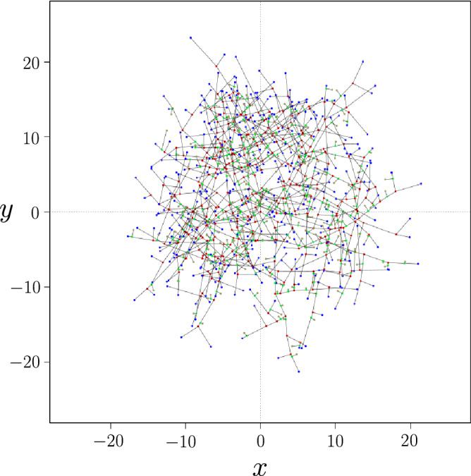
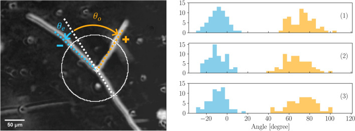
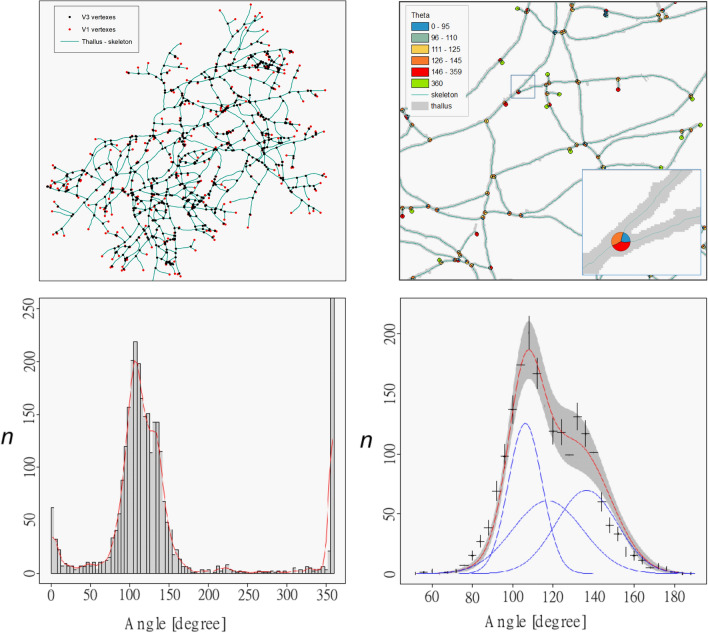
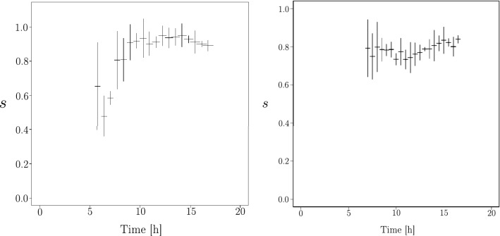
Based upon apical growth and hyphal branching, the two main processes that drive the growth pattern of a fungal network, we propose here a two-dimensions simulation based on a binary-tree modelling allowing us to extract the main characteristics of a generic thallus growth. In particular, we showed that, in a homogeneous environment, the fungal growth can be optimized for exploration and exploitation of its surroundings with a specific angular distribution of apical branching. Two complementary methods of extracting angle values have been used to confront the result of the simulation with experimental data obtained from the thallus growth of the saprophytic filamentous fungus Podospora anserina. Finally, we propose here a validated model that, while being computationally low-cost, is powerful enough to test quickly multiple conditions and constraints. It will allow in future works to deepen the characterization of the growth dynamic of fungal network, in addition to laboratory experiments, that could be sometimes expensive, tedious or of limited scope.

Figure 1

Thallus of P. anserina reconstructed from $8\times 14$ tiles, extracted from experiment 15 h past the ascospore germination (see the text and Table 2 for more details).

Figure 2

Definitions used in this work. The thick line is the mother hypha, while the thin lines are the daughter hyphae. We consider two types of three degrees vertices. $V_{3\ell }$ are lateral branchings, connected with the angle ${\theta }^{\prime }$. $V_3$ are apical branchings on which two branches are connected: an operating and an exploratory branch with respective angles ${\theta }_o$ and ${\theta }_e$. $V_1$ (resp. $V_{1\ell }$) are one degree vertices (i.e. apexes) coming from $V_3$ (resp. $V_{3\ell }$).

Figure 3

Final state (after nine generations) of simulated network for a set of standard parameters. Apical branching led to $N_{V_1}=384$ apexes (shown in blue) and $N_{V_3}=383$ vertices (in red). Lateral branching led to $N_{V_3\ell }=295$ vertices (in green) and $N_{V_1\ell }=295$ apexes (in grey). The spatial dimension in the representation is arbitrary.

Figure 4

Logarithmic distribution (z-direction) of the number of times the branches intersects each other in the network as a function of branch angles ${\theta }_o$ (y-direction) and ${\theta }_e$ (x-direction) in degree for a fixed time and length.

Figure 5

(Left) Typical branching process. A first hypha grows from the bottom right of the image. The branching reveals two new hyphae. A circle of radius $R=80$ $\mathrm{\mu }$m $\sim 5$ hyphal diameters and located on the branching point is drawn. Small angles ${\theta }_e$ and wide angles ${\theta }_o$ are defined by the intersections of this circle with the new hyphae and the projection of the first (mother) hypha. Following the convention proposed into the text, ${\theta }_o>0$ and in this example ${\theta }_e<0$. (Right) (1), (2) and (3) are representations (pdf) of the populations of 66 measurements of the small angle ${\theta }_e$ (in blue) and the wide angle ${\theta }_o$ (in orange), defined in regard to the extension of the mother hypha, see the image on the left for details. Bin width is 4° in this representation. Gaussian fit lead to respective means for small angle $-8.5\pm 4.2$, $-10.2\pm 4.2$ and $-9.2\pm 4.2$, and for wide angle $72.6\pm 4.1$, $67.1\pm 4.3$ and $73.2\pm 4.2$.

Figure 6

(Top-left) Skeletonization of the thallus, with identification of $V_{1ob}$ (red) and $V_{3ob}$ (black) vertices. (Top-right) Automatic calculation of angles from five-pixel buffers around vertices. (Bottom-left) Total angular spectrum with GIS method of the vertices (four populations, three angles from $V_{3ob}$ vertices and one $V_{1ob}$ vertices). (Bottom-right) Zoom in the range of interest. In blue, the three Gaussian distributions. In red the normalised sum of the three Gaussians. In grey, range of one-standard deviation derived from the fit.

Figure 7

Left, one-standard deviation range of the experimental data fit of $V_{1ob}$ (grey) versus time, points: number of $V_{1ob}$ coming from the simulation (black) with scaled time. Right, one-standard deviation range of the experimental data fit of $V_{3ob}$ (grey) versus time, points: number of $V_{3ob}$ coming from simulation (black) with scaled time to the data obtained from $V_{1ob}$. See text for details.

Figure 8

(Left) One standard deviation range of $r_1^{\mathit{data}}$ experimental data fit in function of time (grey). Black points are $r_1^{\mathit{sim}}$ extracted from the simulation with scaled time ans scaled space. (Right) One standard deviation range of $r_3^{\mathit{data}}$ experimental data fit (grey). Black points are $r_3^{\mathit{sim}}$ extracted from the simulation with scaled time and space coming from $V_{1ob}$. See text for details.

Figure 9

Sphericity of $V_{1ob}$ vertices distribution, defined as the ratio $s=2{\lambda }_2/({\lambda }_1+{\lambda }_2)$ of the eigenvalues (see the text for more details) in function of time. Right, sphericity extracted from the simulation, with scaled time and space. Left, is sphericity extracted from experimental data.

Figure 10

Number of apexes $N_{V_{1ob}}$, Number of nodes $N_{V_{3ob}}$ and total length L as a function of time t for the experiments (1) (left), (2) (middle) and (3) (right). Experimental data (blue) are shifted in time of respective $t_0$. Solid black lines represent the best fit parameters (see Table 2). The respective grey shadowing wraps the data range used to perform to statistical fit, while its thickness quantifies the associated uncertainties to one standard deviation.

Figure 11

Skeletonization processes of the thallus. (a) Construction of Thiessen polygons and generation of thallus vertices. (b) Zoom in the left part of (a) shows the point-features vertices of the thallus; Thiesson polygons inside the thallus; the first set of centerlines kept is represented in purple. (c) Final geomatic treatments providing the skeleton (green) after the trimming of the short surrounding line segments (the orange ones).

References

1. Fricker MD, Heaton LLM, Jones NS, Boddy L. The mycelium as a network. Microbiol. Spectrum. 2017 doi: 10.1128/microbiolspec.FUNK-0033-2017. - DOI - PMC - PubMed
1. Sanati Nezhad A, Naghavi M, Packirisamy M, Bhat R, Geitmann A. Quantification of cellular penetrative forces using lab-on-a-chip technology and finite element modeling. Proc. Natl. Acad. Sci. USA. 2013;110:8093–8098. doi: 10.1073/pnas.1221677110. - DOI - PMC - PubMed
1. Boswell GP, Jacobs H, Davidson FA, Gadd GM, Ritz K. Functional consequences of nutrient translocation in mycelial fungi. J. Theor. Biol. 2002;217:459–477. doi: 10.1006/jtbi.2002.3048. - DOI - PubMed
1. Lew RR. How does a hypha grow? The biophysics of pressurized growth in fungi. Nat. Rev. Microbiol. 2011;9:509–518. doi: 10.1038/nrmicro2591. - DOI - PubMed
1. Heaton L, et al. Analysis of fungal networks. Fungal Biol. Rev. 2012;26:12–29. doi: 10.1016/j.fbr.2012.02.001. - DOI
Publication types