Environmental Noise and Effects on Sleep: An Update to the WHO Systematic Review and Meta-Analysis

Abstract

Background: Nighttime noise carries a significant disease burden. The World Health Organization (WHO) recently published guidelines for the regulation of environmental noise based on a review of evidence published up to the year 2015 on the effects of environmental noise on sleep.

Objectives: This systematic review and meta-analysis will update the WHO evidence review on the effects of environmental noise on sleep disturbance to include more recent studies.

Methods: Investigations of self-reported sleep among residents exposed to environmental traffic noise at home were identified using Scopus, PubMed, Embase, and PsycINFO. Awakenings, falling asleep, and sleep disturbance were the three outcomes included. Extracted data were used to derive exposure-response relationships for the probability of being highly sleep disturbed by nighttime noise [average outdoor A-weighted noise level ($L_{\text{night}}$) 2300-0700 hours] for aircraft, road, and rail traffic noise, individually. The overall quality of evidence was assessed using Grading of Recommendations, Assessment, Development, and Evaluations (GRADE) criteria.

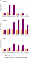
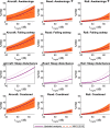
Results: Eleven studies ($n=\mathrm{109,070}$ responses) were included in addition to 25 studies ($n=\mathrm{64,090}$ responses) from the original WHO analysis. When sleep disturbance questions specifically mentioned noise as the source of disturbance, there was moderate quality of evidence for the probability of being highly sleep disturbed per 10-dB increase in $L_{\text{night}}$ for aircraft [$\text{odds ratio}\left(\text{OR}\right)=2.18$; 95% confidence interval (CI): 2.01, 2.36], road ($\text{OR}=2.52$; 95% CI: 2.28, 2.79), and railway ($\text{OR}=2.97$; 95% CI: 2.57, 3.43) noise. When noise was not mentioned, there was low to very low quality of evidence for being sleep disturbed per 10-dB increase in $L_{\text{night}}$ for aircraft ($\text{OR}=1.52$; 95% CI: 1.20, 1.93), road ($\text{OR}=1.14$; 95% CI: 1.08, 1.21), and railway ($\text{OR}=1.17$; 95% CI: 0.91, 1.49) noise. Compared with the original WHO review, the exposure-response relationships closely agreed at low (40 dB $L_{\text{night}}$) levels for all traffic types but indicated greater disturbance by aircraft traffic at high noise levels. Sleep disturbance was not significantly different between European and non-European studies.

Discussion: Available evidence suggests that transportation noise is negatively associated with self-reported sleep. Sleep disturbance in this updated meta-analysis was comparable to the original WHO review at low nighttime noise levels. These low levels correspond to the recent WHO noise limit recommendations for nighttime noise, and so these findings do not suggest these WHO recommendations need revisiting. Deviations from the WHO review in this updated analysis suggest that populations exposed to high levels of aircraft noise may be at greater risk of sleep disturbance than determined previously. https://doi.org/10.1289/EHP10197.

Figure 1.

Flow diagram of study identification, screening, and selection. “Study” refers to a data collection campaign including a defined group of participants and one or more outcomes. In one instance, a study was reported in multiple articles^, and is counted as $n=1$ study. “Report” is a journal article, preprint, conference abstract, study register entry, clinical study report, dissertation, unpublished manuscript, government report, or other document supplying relevant information about a particular study or studies.

Figure 2.

Effective sample sizes for (A) aircraft, (B) road, and (C) rail for each sleep disturbance question in the present updated analysis, determined from the original WHO analysis plus the 11 newly included studies, compared with sample sizes from the WHO 2018 review only. Note: WHO, World Health Organization.

Figure 3.

Forest plot for the odds of being highly sleep disturbed by aircraft noise per 10-dB increase in $L_{\text{night}}$ (combined estimate derived from all relevant outcomes within studies). Subgroups are presented for questions that mentioned noise as the source of the disturbance, and questions that did not specify noise as the source of the disturbance. Risk of bias: A: selection bias; B: exposure assessment; C: confounding; D: reporting bias. Green ($+$) denotes low risk of bias, red (–) denotes high risk of bias, yellow (?) denotes unclear risk of bias. Plots were generated using an inverse-variance (IV) random effects method across the full noise range for each individual study (not restricted to 40–65 dB $L_{\text{night}}$). Note: CI, confidence interval; df, degrees of freedom; $L_{\text{night}}$, nighttime noise; NORAH, Noise-Related Annoyance, Cognition and Health.

Figure 4.

Forest plot for the odds of being highly sleep disturbed by road noise per 10-dB increase in $L_{\text{night}}$ (combined estimate derived from all relevant outcomes within studies). Subgroups are presented for questions that mentioned noise as the source of the disturbance, and questions that did not specify noise as the source of the disturbance. Risk of bias: A: selection bias; B: exposure assessment; C: confounding; D: reporting bias. Green ($+$) denotes low risk of bias, red (–) denotes high risk of bias, yellow (?) denotes unclear risk of bias. Plots were generated using an inverse-variance (IV) random effects method across the full noise range for each individual study (not restricted to 40–65 dB $L_{\text{night}}$). Note: CI, confidence interval; df, degrees of freedom; $L_{\text{night}}$, nighttime noise; NORAH, Noise-Related Annoyance, Cognition and Health.

Figure 5.

Forest plot for the odds of being highly sleep disturbed by railway noise per 10-dB increase in $L_{\text{night}}$ (combined estimate derived from all relevant outcomes within studies). Subgroups are presented for questions that mentioned noise as the source of the disturbance, and questions that did not specify noise as the source of the disturbance. Risk of bias: A: selection bias; B: exposure assessment; C: confounding; D: reporting bias. Green ($+$) denotes low risk of bias, red (–) denotes high risk of bias, yellow (?) denotes unclear risk of bias. Plots were generated using an inverse-variance (IV) random effects method across the full noise range for each individual study (not restricted to 40–65 dB $L_{\text{night}}$). Note: CI, confidence interval; $L_{\text{night}}$, nighttime noise; NORAH, Noise-Related Annoyance, Cognition and Health.

Figure 6.

Probability of being highly sleep disturbed (%HSD) by nighttime noise, determined via questions that mention noise as the source of disturbance, stratified by disturbance question and traffic mode. Exposure–response relationships were derived using all available data, from the original WHO review and the 11 newly identified studies. Results of the present updated analysis (solid purple lines with dotted 95% CIs) are compared against results of the 2018 WHO review (dashed orange lines with shaded 95% CIs). Relationships for the sleep disturbance questions were not calculated previously. Asterisks (*) indicate sleep outcomes for which no new studies have been published since the WHO review. Parameter estimates were calculated in logistic regression models with $L_{\text{night}}$ included as the only fixed effect and study included as a random effect, restricted to the noise exposure range 40–65 dB $L_{\text{night}}$. Models were run separately for each traffic mode and disturbance question. The combined estimate was calculated using average responses of the awakening, falling asleep, and sleep disturbance questions within studies. Note: CI, confidence interval; $L_{\text{night}}$, nighttime noise; WHO, World Health Organization.

Figure 7.

Exposure–response relationships for the probability of being highly sleep disturbed (%HSD) by nighttime noise for questions that mention noise. Curves are shown for the updated analysis that includes all available data (solid purple lines), and for analysis including only newly identified studies published after the WHO review (dashed green lines). Data are calculated as the combined response using average responses of the awakening, falling asleep, and sleep disturbance questions within studies, determined as the within-study average of disturbance questions that explicitly mentioned noise as the source of sleep disturbance. Parameter estimates were calculated in logistic regression models with $L_{\text{night}}$ included as the only fixed effect and study included as a random effect, restricted to the noise exposure range 40–65 dB $L_{\text{night}}$. Models were run separately for each traffic mode. Note: $L_{\text{night}}$, nighttime noise; WHO, World Health Organization.

Figure 8.

Probability of being highly sleep disturbed (%HSD) by nighttime noise, determined via questions that did not specifically mention noise as the source of disturbance, stratified by disturbance question and traffic mode. Exposure–response relationships were derived using all available data, from the original WHO review and the 11 newly identified studies. Dotted lines indicate 95% CIs. Parameter estimates were calculated in logistic regression models with $L_{\text{night}}$ included as the only fixed effect and study included as a random effect, restricted to the noise exposure range 40–65 dB $L_{\text{night}}$. Models were run separately for each traffic mode and disturbance question. The combined estimate was calculated using average responses of the awakening, falling asleep, and sleep disturbance questions within studies. Note: CI, confidence interval; $L_{\text{night}}$, nighttime noise; WHO, World Health Organization.