Dynamical landscapes of cell fate decisions

Abstract

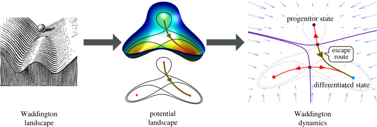
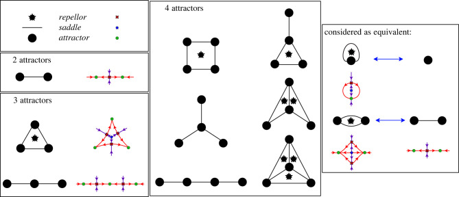
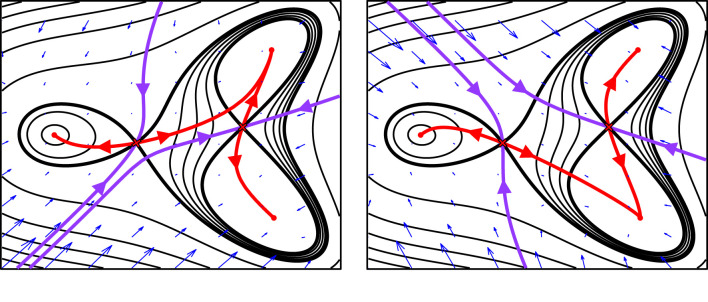
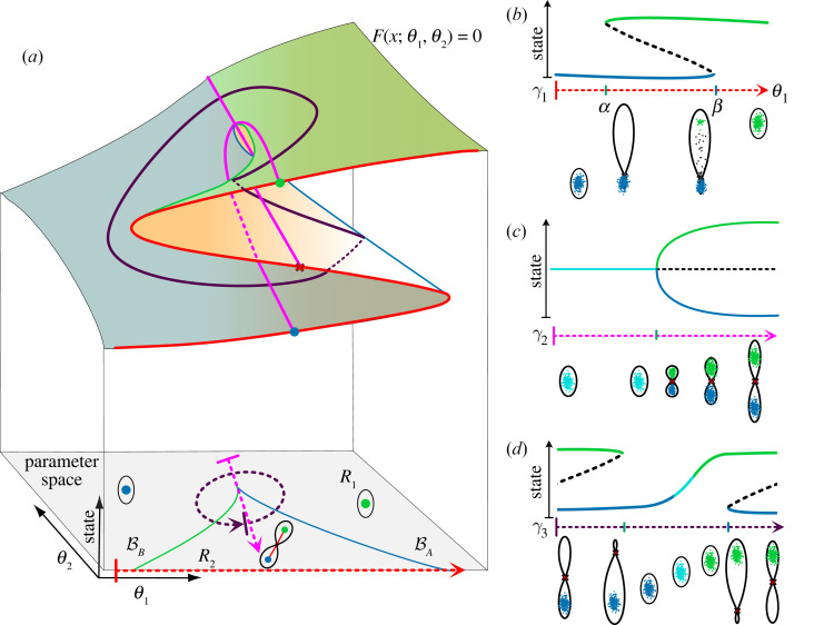
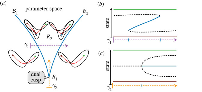
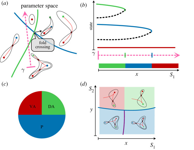
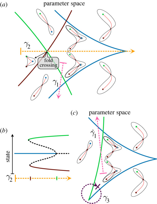
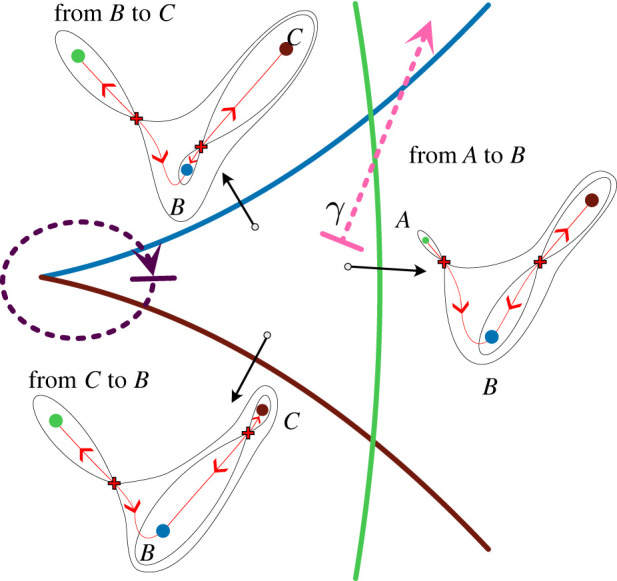
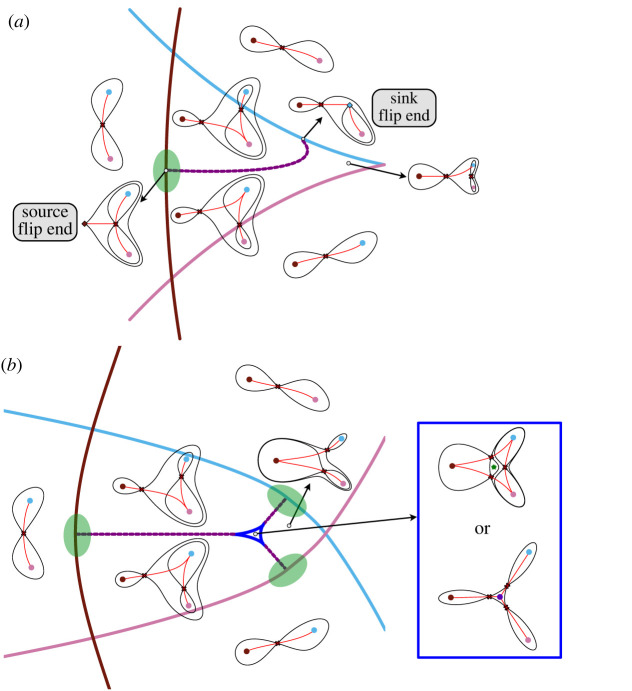
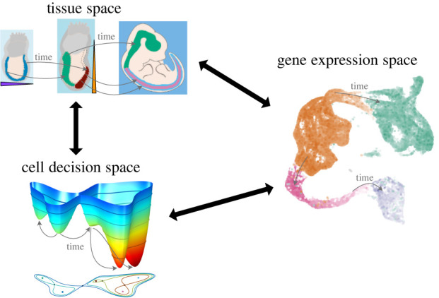
The generation of cellular diversity during development involves differentiating cells transitioning between discrete cell states. In the 1940s, the developmental biologist Conrad Waddington introduced a landscape metaphor to describe this process. The developmental path of a cell was pictured as a ball rolling through a terrain of branching valleys with cell fate decisions represented by the branch points at which the ball decides between one of two available valleys. Here we discuss progress in constructing quantitative dynamical models inspired by this view of cellular differentiation. We describe a framework based on catastrophe theory and dynamical systems methods that provides the foundations for quantitative geometric models of cellular differentiation. These models can be fit to experimental data and used to make quantitative predictions about cellular differentiation. The theory indicates that cell fate decisions can be described by a small number of decision structures, such that there are only two distinct ways in which cells make a binary choice between one of two fates. We discuss the biological relevance of these mechanisms and suggest the approach is broadly applicable for the quantitative analysis of differentiation dynamics and for determining principles of developmental decisions.

Keywords: Waddington landscape; bifurcations; cellular decision-making; development; dynamical systems.

Figure 1.

From Waddington’s landscapes to Waddington dynamics. The classic picture of a Waddington landscape (left) can be formalized using a potential function (middle). Nevertheless, to capture the full behaviour of the system complete Waddington dynamics are needed (right). The dynamics describe the trajectories cells take between different states.

Figure 2.

Two-dimensional landscapes. (a) System with three attractors and two saddles. The purple curves are the separatrices or stable manifolds of the saddles, the red curves are the unstable manifolds (if time is run backwards points on these converge to the saddle). Points on each unstable manifold converge to two attractors and the stable manifolds divide the phase space into three basins, one for each attractor. Level curves for the saddles are indicated in black. (b) Saddle point. The dynamics near a saddle point. The stable (purple) and unstable (red) manifolds are shown.

Figure 3.

Binary decisions. (a) Binary choice landscape. In the starting condition, Signal 1, cells are in a progenitor state corresponding to the middle basin of the landscape. Exposure to Signal 2 results in the disappearance of the central basin and the bottom ridge and cells transition into State B following the slopes of the new landscape. (b) Two parameters p₁ and p₂ govern the landscape in (a). Bifurcations occur when these parameters are on the black curves in p₁, p₂-space. Crossing one curve results in cells transitioning to A; crossing the other, cells transition to B. (c) Binary flip landscape. Cells start in the progenitor state P which corresponds to a shallow basin. Noise is sufficient for cells to transition into the more committed states and they follow the escape route (red) towards state A when exposed to Signal 1. In response to Signal 2 the escape route flips towards B and cells transition towards B. (d) The landscape in C is also governed by two parameters. The progenitor attractor is destroyed when the parameters are on the black curve and the flip occurs when the parameters are on the purple curve.

Figure 4.

Fold bifurcation. Representation of a landscape before (left) a fold bifurcation, at the bifurcation point (middle) and beyond it (right). The attractor and saddle collide and disappear (middle) so cells in that basin of attraction follow the escape route (red) to another attractor.

Figure 5.

Decision structures with up to four attractors. Nodes correspond to attractors and edges to saddles with unstable manifolds that connect the corresponding attractors. The asterisks denote the existence of at least one saddle of index 2. In 2D systems such a saddle is a repellor.

Figure 6.

The potential alone does not determine the dynamics. Two qualitatively different dynamical systems that have exactly the same landscape potential. The potential, alone, does not determine the position of the unstable manifolds of the saddles and therefore does not determine to which attractor transitioning cells go. In a gradient system using the standard Riemannian metric (see box 2) the trajectories are always perpendicular to the contours but this does not have to be the case. Dynamical systems that flow downhill, from higher altitude to lower, can cross the contours at angles other than ${90}^{\circ }$ (see box 2). In this example, we show a modification that produces a flip in the unstable manifold of the saddle. This example shows that the potential does not determine the decision structure.

Figure 7.

Bistability: the standard cusp. (a) Catastrophe manifold and bifurcation set. In 2D parameter space, the blue and green lines represent the bifurcation set with the colour of the line corresponding to the attractor involved in the fold bifurcation that occurs on that fold line. The dashed arrows indicate example paths in parameter space, corresponding to a continuous change in an extrinsic signal. The 2D catastrophe manifold on top of the parameter space shows the fold lines and the preimages of the different paths that are sketched with more detail in panels (b,c,d). In the region R₂ (inside the cusp, with three sheets above), there are two attractors A and B separated by a saddle S. When the parameters move out of R₂ to R₁ (outside the cusp, with one sheet above) by crossing ${\mathcal{B}}_A$ (respectively, ${\mathcal{B}}_B$) the attractor A (respectively, B) and the saddle undergo a fold bifurcation which destroys A (respectively, B). Paths γ₁ across the cusp, γ₂ vertically through the cusp, and γ₃ around the cusp correspond to the hysteresis, pitchfork and cusp smooth swap diagrams (respectively). (b) Bifurcation diagram of a genetic switch. Change in the rest points of a bistable system, as a parameter θ₁ changes. A single attractor (green) is present when θ = 0. When θ₁ crosses the bifurcation point (α), a saddle (dashed curve) and a new attractor (blue) appear. When the parameter crosses a second bifurcation point (β) the initial attractor (green) collides with the saddle and disappear causing the cells in it to transition to the available attractor (blue). The coexistence of both attractors between α and β results in bistability and hysteresis. (c) Pitchfork. As a parameter changes along γ₂, an initial attractor becomes a saddle point and two attractors appear at each side. The system is symmetric with respect to the saddle point. (d) Smooth state swap. The path γ₃ around the cusp shows how cells transition from A into B without a step-like switch. When the path crosses the bifurcation set, the bifurcating attractor is empty and hence no cells are forced to transition, instead, going around the cusp in R₁ changes the gene expression in a smooth continuous way.

Figure 8.

The choice landscape: the dual cusp. (a) Bifurcation set. The solid lines show the bifurcation set. The dashed arrow shows a path in parameter space. In the region R₂ (inside the cusp, above), there are three attractors separated by two saddles. When the parameters move out of R₂ to R₁ (outside the cusp, below) by crossing ${\mathcal{B}}_1$ (respectively, ${\mathcal{B}}_2$) the central attractor (blue) and the right (respectively, left) saddle undergo a fold bifurcation which destroys the attractor. (b) The path (γ₁) indicated gives a 1D representation of the choice family and the available transitions from the central attractor. The duality between the hysteresis diagram and the middle part of this diagram is apparent. (c) The path (γ₂) indicated shows a pitchfork bifurcation where the central saddle becomes two saddles and a new attractor. The duality between this diagram and figure 7c is apparent.

Figure 9.

Fold crossing points of bifurcation curves. (a) Bifurcation set. Landscapes around a fold crossing, corresponding to two adjacent attractors, one central (blue), the others peripheral (green, red). The solid lines represent the bifurcation set with the colour of the line corresponding to the bifurcating attractor. (b) French flag model. The path γ in the 2D parameter space in (a) produces the bifurcation diagram shown in (b). Suppose that the cells are spatially organized in 1D with coordinate x and all cells start in the green attractor. Cells are exposed to a signal S(x) which increases monotonically with x. If x is small so that the signal is small, cells will stay in the green attractor. For larger values of x which will have higher values of the signal, the cells will transition to the blue or red attractor. Moreover, cells will stay in the attractor when the signal decreases. Since the signal is a monotonic function of x this results in a French flag pattern. (c,d) Meinhardt boundary model. When there are two signals, a landscape with a flip curve endpoint as in (d) can produce patterning in a similar fashion. In such an arrangement, a system transitions between three states in response to a combination of two signals. In this model the physical space of the tissue is 2D: one dimension, x, has a gradient of signal S₁ and the other, y, has a graded signal S₂. All cells are assumed to start in the blue attractor. If signal S₂ is small enough that the point (x, y) is below the blue fold curve of the bifurcation set, then the cell stays in this attractor. If (x, y) is above the fold curve this attractor is destroyed in a fold bifurcation and the cells transition to one of the other attractors. Because of the flip, when (x, y) is in the red region (respectively, green region) the state transition to the red (respectively, green) attractor. Moreover, all cells stay in the respective attractor when the signal S₂ decreases. Consequently, after a pulse of the signals the spatial patterning is as shown in (c) with three distinct regions of tissue.

Figure 10.

Families with a dual cusp. (a,c) Bifurcation sets. Two landscape families with a dual cusp. The solid lines show the bifurcation set with the colour of the line corresponding to the attractor involved in the fold bifurcation. The dashed arrows illustrate paths in parameter space. (a) The region where there are three attractors is bounded by a dual cusp and fold curves with crossings. The crossings that can occur are highly constrained [2]. Path γ₁ corresponds to a French flag landscape. (b) Symmetry breaking. This bifurcation diagram corresponds to the path γ₂ in (a). It is the dual cusp version of the pitchfork bifurcation that occurs in the standard cusp. Like the pitchfork, it is not generic but in the exceptional case where there is a ${\mathbb{Z}}_2$-symmetry such as when the system describes the behaviour of two identical cells it becomes generic and describes an interesting symmetry breaking bifurcation (see [24] for an example). (c) A three attractor region bounded by a dual and standard cusp. Path $\widehat{{\gamma }_1}$ corresponds to the French flag landscape. Path γ₃ corresponds to the cusp smooth state swap of the green and blue attractors.

Figure 11.

Families with one standard cusp and no other cusps. The landscape family with the solid lines representing the bifurcation set. The colour of the line corresponds to the attractor involved in the fold bifurcation. Path γ corresponds to a French flag landscape. A cusp smooth state swap path is also sketched.

Figure 12.

Families with flip curves. (a,b) Bifurcation sets. The bifurcation sets for two landscape families: the solid lines indicate fold curves and the dashed lines are flip curves. The colour of the fold line corresponds to the attractor involved in the fold bifurcation. Examples of landscapes in the family are sketched. Both families contain the flip landscape in the areas marked in green. (a) One flip with a cusp. The two attractors connected to the sink saddle can undergo a cusp bifurcation. (b) With no cusps. This family contain three instances of the flip landscape. The region enclosed by the blue deltoid corresponds to landscapes with an extra pair of critical points: a saddle and either a repellor or an attractor (as shown in the blue box). Generically, the flip curves enter the deltoid avoiding the cusps and terminate in one of the three smooth edges of the deltoid. This family is part of the compactified elliptic umbillic catastrophe.

Figure 13.

Three developmental spaces. A developing cell can be followed through three distinct spaces. The location of a cell in tissue space gives the coordinates of a cell in a developing embryo and indicates the signalling environment to which it is exposed. The same cell can also be represented in gene expression space by its molecular identity. In addition, the cell occupies a position within cell decision space. This is the location in a Waddington dynamics landscape, which represents its cell fate and describes the decision-making process. The goal is to be able to link cells in these three spaces and to map how a cell moves through them over time.

References

1. Waddington C. 1957. The strategy of the genes. London, UK: Allen & Unwin.
1. Rand DA, Raju A, Saez M, Corson F, Siggia ED. 2021. Geometry of gene regulatory dynamics. Proc. Natl Acad. Sci. USA 118, 15. (10.1073/pnas.2109729118) - DOI - PMC - PubMed
1. Smale S. 1967. Differentiable dynamical systems. Bull. Am. Math. Soc. 73, 747-817. (10.1090/S0002-9904-1967-11798-1) - DOI
1. Thom R. 1989. Structural stability and morphogenesis: an outline of a general theory of models. Boca Raton, FL: CRC Press.
1. Zeeman EC. 1977. Catastrophe theory: selected papers, 1972–1977. Advanced Book Program. Reading, MA: Addison-Wesley.
LinkOut - more resources