. 2022 Jul 21:11:e80470.
doi: 10.7554/eLife.80470.

Mapping odorant sensitivities reveals a sparse but structured representation of olfactory chemical space by sensory input to the mouse olfactory bulb

Affiliations

Mapping odorant sensitivities reveals a sparse but structured representation of olfactory chemical space by sensory input to the mouse olfactory bulb

Shawn D Burton et al. Elife. .

Abstract

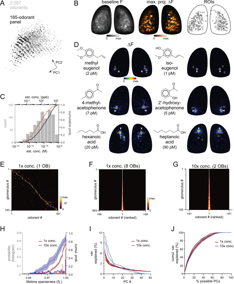
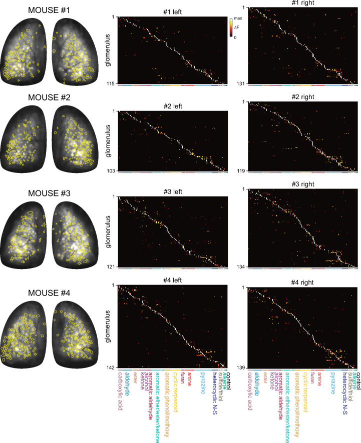
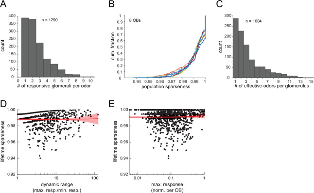
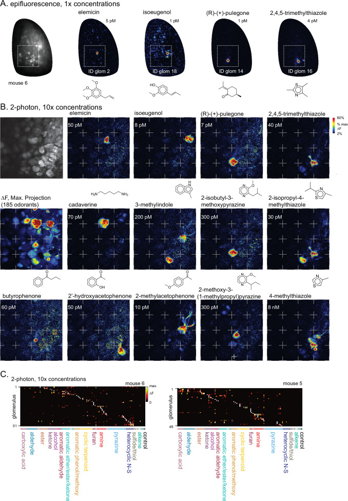
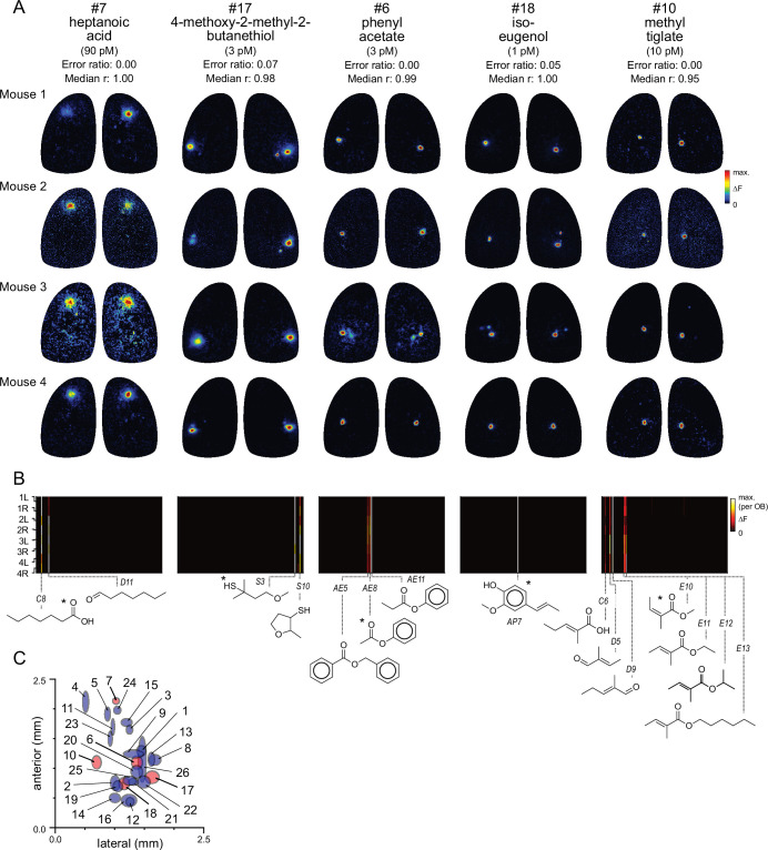
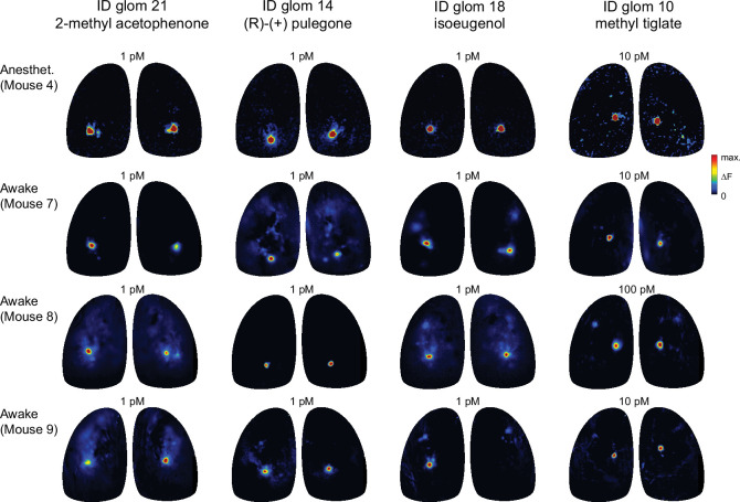
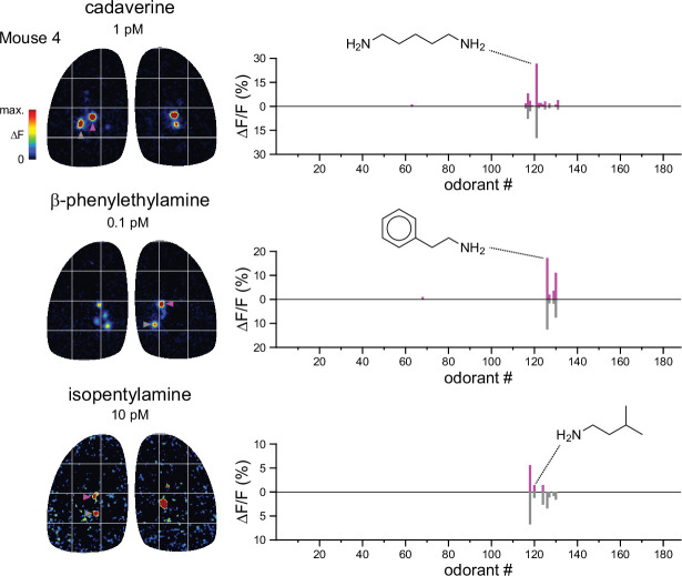
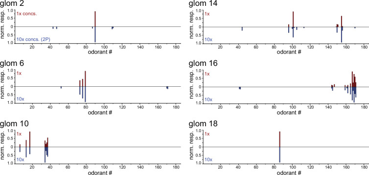
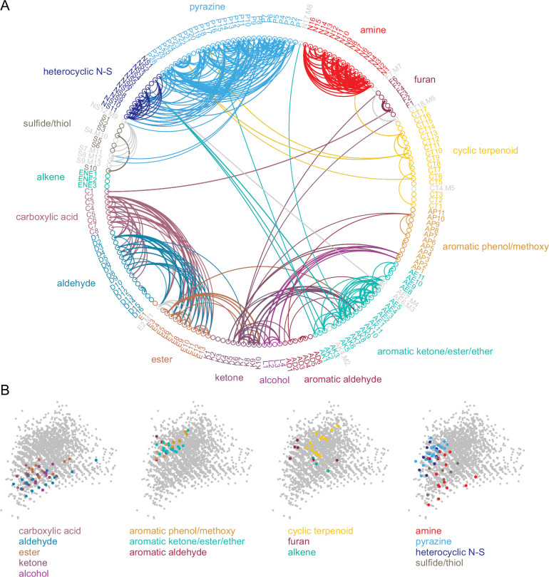
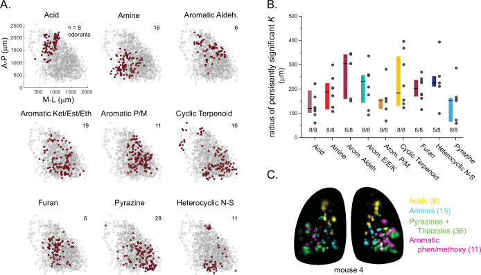
In olfactory systems, convergence of sensory neurons onto glomeruli generates a map of odorant receptor identity. How glomerular maps relate to sensory space remains unclear. We sought to better characterize this relationship in the mouse olfactory system by defining glomeruli in terms of the odorants to which they are most sensitive. Using high-throughput odorant delivery and ultrasensitive imaging of sensory inputs, we imaged responses to 185 odorants presented at concentrations determined to activate only one or a few glomeruli across the dorsal olfactory bulb. The resulting datasets defined the tuning properties of glomeruli - and, by inference, their cognate odorant receptors - in a low-concentration regime, and yielded consensus maps of glomerular sensitivity across a wide range of chemical space. Glomeruli were extremely narrowly tuned, with ~25% responding to only one odorant, and extremely sensitive, responding to their effective odorants at sub-picomolar to nanomolar concentrations. Such narrow tuning in this concentration regime allowed for reliable functional identification of many glomeruli based on a single diagnostic odorant. At the same time, the response spectra of glomeruli responding to multiple odorants was best predicted by straightforward odorant structural features, and glomeruli sensitive to distinct odorants with common structural features were spatially clustered. These results define an underlying structure to the primary representation of sensory space by the mouse olfactory system.

Keywords: chemoinformatics; coding; imaging; mouse; neuroscience; odor; olfactometry.


Conflict of interest statement

SB, AB, TE, IY, TR, MS, MW No competing interests declared

Figures

Figure 1.
Figure 1.. High sensitivity and narrow tuning of olfactory sensory input to OB glomeruli.
(A) Coverage of physicochemical space by the 185-odorant panel. Grey points show the projection of 2,587 odorants across the first two principal components of a matrix of physicochemical descriptors, as in Pashkovski et al., 2020 (see Materials and methods). Black points indicate the odorants tested in the 185-odorant panel. (B) Baseline fluorescence (left), maximal projection of response maps across the 185-odorant panel (middle), and ROIs of responsive glomeruli (right). (C) Estimated delivered concentrations used across the odorant panel. Histogram and black cumulative distribution function show concentrations of each presented odorant across four preparations (n=740). Red cumulative distribution function shows the minimal effective concentration for each responsive glomerulus (n=993). (D) Response maps evoked by single odorants for the preparation shown in (B). Each row shows distinct but neighboring glomeruli (demarcated by filled and open arrowheads) activated by structurally similar odorants. Estimated concentrations are rounded to single-significant digit precision. (E) Matrix of responses across all responsive glomeruli in one OB. Each row (glomerulus) is normalized to its maximal response across the odorant panel. Glomeruli are sorted in order of their maximally-activating odorant, producing a pseudo-diagonalized matrix. Odorants are ordered according to nominal structural classification (see Materials and methods). Matrix includes responses to empty and solvent controls. (F, G) Response spectra of all imaged glomeruli (rows) across the odorant panel (columns), normalized by maximal response, for 1 x concentration epifluorescence dataset and the 10 x concentration two-photon dataset (separate preparations; 10 x two-photon data imaged from a smaller field of view containing fewer glomeruli). Odorant order sorted by response amplitude; glomerular order sorted by lifetime sparseness. (H) Histogram and cumulative distribution functions of lifetime sparseness (SL) values for all responsive glomeruli for the odorant panel presented at original, 1 x concentrations (red; n=993 glomeruli) and at 10 x concentrations (blue; n=100). Shading denotes 95% confidence intervals (calculated using ‘ecdf’ function in Matlab). (I) Percent of variance in glomerular responses to the odorant panel explained by each successive PC, plotted for each OB. Red plots: 1 x concentrations, n=8 OBs; blue plots: 10 x concentrations, n=2 OBs. (J) Cumulative variance in glomerular responses to the odorant panel explained by increasing fractions of possible PCs (constrained by the number of responsive glomeruli in each OB).
Figure 1—figure supplement 1.
Figure 1—figure supplement 1.. Summary of responsive glomeruli and their response spectra.
Left: Overlay of all ROIs indicating odorant-responsive glomeruli (yellow) and baseline fluorescence for the four mice imaged under widefield epifluorescence. Right: Matrices of responses across all responsive glomeruli and odorants in each OB after manual segmentation as described (see Materials and methods). Glomeruli and odorants are sorted as in Figure 1E and odorants occur in the same order as in Supplementary file 1. Naming and color-coding of odorant structural classes matches those in Figures 4 and 5.
Figure 1—figure supplement 2.
Figure 1—figure supplement 2.. Comparison of delivered odorant concentrations across studies.
(A) Pairwise comparison of delivered odorant concentrations in the current study (red circles) vs. select previous studies (black circles). Only odorants common across each pair of studies are plotted, with lines connecting concentrations of the same odorant. (B) Distribution of the delivered concentration of each odorant in previous studies relative to the concentration of the same odorant used in the current study. Numbers of odorants plotted is equal to the number of data points shown in (A). Dashed red line marks equal concentrations across the previous and current study. Boxes show median and interquartile range; whiskers delimit the most extreme values not considered outliers, as defined by the ‘boxplot’ function in Matlab. Both absolute (A) and relative (B) odorant concentrations are shown on a log-scale.
Figure 1—figure supplement 3.
Figure 1—figure supplement 3.. Sparse glomerular responses evoked across the 185-odorant panel.
(A) Histogram of number of glomeruli activated by a given odorant presentation, excluding non-responsive presentations (n=1290, 8 OBs imaged under widefield epifluorescence). (B) Cumulative distribution function of population sparseness (SP) for each odorant, plotted separately for each of the eight OBs. SP of 1 indicates a single responsive glomerulus. (C) Distribution of the number of effective odorants for each of 1004 glomeruli across the eight OBs. (D) Lifetime sparseness (SL) of glomerular tuning across the 185-odorant panel, plotted as a function of dynamic range for all glomeruli responding to more than one odorant (n=716 glomeruli). Dynamic range is conservatively defined as the ratio between the maximal response and the minimal non-zero odorant response. Red plot shows linear regression to data, with 95% confidence interval. Slope is not significantly different from 0 (linear regression t-test: p=0.89, t714=0.14). (E) SL as a function of maximal response amplitude for all imaged glomeruli (n=1004). Responses normalized to the maximal response in a given OB. Red plot shows linear regression to data, as in (D). Slope is not significantly different from 0 (linear regression t-test: p=0.42, t1002=0.81).
Figure 1—figure supplement 4.
Figure 1—figure supplement 4.. Two-photon imaging of glomerular odorant responses to tenfold higher odorant concentrations.
(A) Epifluorescence response maps to 1 x concentrations of diagnostic odorants for functionally-identified glomeruli, imaged across one OB (new mouse, ‘mouse #6’). (B) Higher magnification two-photon imaging of the boxed area in (A) using 10 x odorant concentrations. Upper left, baseline fluorescence of glomerular imaging field. Response maps (ΔF) show activation of specific glomeruli by select odorants. Dashed grid lines added to facilitate visual inspection across maps. (C) Left: Response matrix for glomeruli imaged in (B), showing responses to the 10 x concentration odorant panel for mouse #6. Only responses to odorants tested at 10 x concentration (plus blank and solvent controls) are shown. Glomeruli are sorted in order of their maximally-activating odorant, producing a pseudo-diagonalized matrix, as in Figure 1E. Right: Response matrix for the same 10 x odorant panel imaged in a second mouse (mouse #5).
Figure 2.
Figure 2.. Functional identification of glomeruli using singular activation by diagnostic odorants.
(A) Response maps evoked by five odorants (columns), shown for each of four mice (rows), eliciting singular or near-singular activation of a glomerulus in a consistent location in each OB. See Text for definition of error ratio and median r. Estimated delivered concentrations are rounded to single-significant digit precision. (B) Response spectra for each glomerulus in (A) across the 185-odorant panel (columns), shown for each of the eight imaged OBs (rows). Pseudocolor scale is normalized to the maximal response in the glomerulus for each preparation. Structures of effective odorants are shown at bottom. Asterisk indicates diagnostic odorant shown in (A). Letter-number abbreviations indicate odorant identity, as listed in Supplementary file 1. (C) Mean locations of all functionally identified glomeruli, referenced to the midline and caudal sinus of the OB. Spot width and height indicate jitter (s.d.) of medial-lateral and antero-posterior location across the eight OBs. Identified glomeruli from (A) are shown in red; all other glomeruli shown in blue.
Figure 2—figure supplement 1.
Figure 2—figure supplement 1.. Diagnostic odorants functionally identify glomeruli with similar sensitivity in awake mice.
Comparison of response maps evoked by diagnostic odorants for four functionally-identified glomeruli in an anesthetized mouse (Mouse #4, top row) and in three awake, head-fixed mice (Mice #7–9). Odorants were prepared and presented identically across anesthetized and awake preparations. Awake response maps are averages of three to five presentations and are scaled as for anesthetized responses. Concentrations indicate estimated delivered concentration, as in previous Figures.
Figure 2—figure supplement 2.
Figure 2—figure supplement 2.. Functional identification of putative TAAR-associated glomeruli using amine odorants.
Left: Response maps for 3 amine odorants previously identified as high-potency ligands for different TAARs (see Text). Each amine most strongly activates different paired glomeruli on each OB, highlighted by magenta and grey arrowheads. Right: Response spectra for each of the paired glomeruli for each amine; the vertical axis for the posterior glomerulus is inverted for easier visual comparison. The response spectra are near-identical for each of the paired glomeruli, and distinct for each pair.
Figure 2—figure supplement 3.
Figure 2—figure supplement 3.. Identified glomeruli maintain narrow tuning across a tenfold increase in odorant concentrations.
Response spectra of six functionally-identified glomeruli evoked by the original 185-odorant panel (1 x concentrations, top, red bars) and by the same odorants presented at tenfold higher concentrations (10 x, bottom, blue bars), imaged in separate preparations under widefield epifluorescence and two-photon imaging, respectively. 1 x plots show median response spectrum across the eight imaged OBs. 10 x plots show mean responses from two imaged OBs (two mice) (for glomeruli 2, 14, 18); or from a single OB (for glomeruli 6, 10, 16), each normalized to the maximum response across the odorant panel.
Figure 3.
Figure 3.. Predicting odorant response specificity from physicochemical feature sets.
(A) Median response spectra of all functionally-identified glomeruli. Each spectrum (row) is normalized to its maximal odorant response. Odorants ordered according to nominal structural classification (see Materials and methods), as in Figure 1E. (B) Median response spectra of functionally-identified glomeruli, with odorants ordered by physicochemical descriptor distance from the primary odorant for each glomerulus (odorant that evokes a response at the lowest concentration), using the Dragon1377 descriptor set. (C) Cumulative fraction of all odorant responses encountered with increasing ranked distance from the primary odorant, averaged across all 19 functionally identified glomeruli with co-tuning (i.e. responding to more than one odorant). Colored lines show the cumulative response fraction observed for different odorant rankings, including distance in: the Dragon1377 descriptor set (as shown in (B)), the Dragon1377 descriptor set re-ordered relative to the strongest-activating odorant (Dragon1377 (max)), and a larger 2982-element descriptor set (Alvad. 2982). Black line shows the cumulative response fraction of binarized odorant responses, with odorants ranked by response magnitude, representing the maximum achievable response prediction by odorant ranking. Grey lines show cumulative response fraction following random odorant ranking (100 iterations), representing chance prediction. (D) Same as (C) for all co-tuned glomeruli imaged across the eight OBs (n=694), relative to the primary odorant for each glomerulus, for different odorant rankings, including distance in: the Dragon1377 descriptor set, a previously optimized subset of 32 Dragon descriptors (Dragon32), a subset of descriptors defining functional groups (FG(49)), a subset of previously developed chemical feature binarized fingerprints (i.e. bits; MACCS(106)), and a novel set of chemical feature binarized fingerprints (SMARTS42). Grey line shows mean cumulative response fraction following random odorant ranking. (E) Distribution of performance metrics (see Materials and methods; 1 indicates perfect prediction, 0 indicates chance prediction) across all 694 co-tuned glomeruli for different odorant rankings. Red bar, median; Center bar, interquartile range; envelope, smoothed point density. Asterisks indicate significant difference between odorant rankings (Kruskal-Wallis test comparing all performance metrics: p<2 × 10–16; chi-squared statistic, 859; df = 6; p=0.002 for MACCS(106) vs. Dragon32; p<1 × 10–25 for MACCS(106) vs. all other rankings (post-hoc Dunn tests, Benjamani-Hochberg correction for multiple comparisons); only differences between incrementally higher medians are shown for clarity). (F) Prediction performance metrics for each of the 694 co-tuned glomeruli for the 32-element optimized Dragon descriptor subset (Dragon32; black points) and the 42-element SMARTS fingerprints (SMARTS42; red points), with glomeruli ordered by Dragon32 performance.
Figure 3—figure supplement 1.
Figure 3—figure supplement 1.. Additional comparisons of glomerular response predictions by physicochemical descriptor sets.
(A) Median response spectra of functionally identified glomeruli, with odorants ordered by physicochemical descriptor distance from the strongest-activating odorant for each glomerulus, using the Dragon1377 descriptor set (compare with ordering relative to primary odorant, Figure 3B). (B) Median response spectra of functionally-identified glomeruli, with odorants ordered relative to distance in the space defined by the first 20 PCs of the space defined by the 2982-element alvadesc physicochemical descriptors applied to 2,624 odorant compounds in the Good Scents odorant database (see Text). (C) Median response spectra of functionally-identified glomeruli, with odorants ordered relative to distance (dice similarity) from the primary odorant using the SMARTS42 fingerprint. (D) Cumulative variance in the 2982-descriptor x 2624-odorant space explained by successive PCs (blue line), overlaid with mean prediction performance of 694 co-tuned glomerular responses by odorant ranking using increasing numbers of 2982-descriptor x 2624-odorant space PCs. The first 20 PCs explain 66% of the variance in the 2982-descriptor x 2624-odorant space, while prediction performance asymptotes at ~0.6 after 5–10 PCs. (E) Comparison of prediction performance scores for each of the 694 co-tuned glomeruli for the Dragon1377 descriptor set (black points) and the SMARTS42 set (red points), with glomeruli ordered by Dragon1377 performance. (F) Comparison of MACCS (black points) and SMARTS42 performance scores (red points) for the same 694 co-tuned glomeruli.
Figure 4.
Figure 4.. Sparse tuning of glomerular inputs is heterogeneously structured.
(A) Mean glomerular response correlation matrix for the 185-odorant panel. Each value shows the Spearman’s rank correlation (ρ) between the vectors of glomerular responses evoked by two odorants, averaged across all 8 OBs. Odorants ordered and color-coded according to nominal structural classification (see Materials and methods), as in Figure 1E. (B) Odorant co-tuning probability matrix for the 185-odorant panel. Each value shows the mean probability of a glomerulus responding to each odorant pair of the matrix, averaged across all responsive glomeruli per OB and then averaged across each of the eight OBs.
Figure 5.
Figure 5.. Odorant co-tuning relationships reflect basic chemical features of odorants.
(A) Circular network graph of the most reliable odorant co-tuning relationships, using the mean number of glomeruli co-tuned to each odorant pair. Lines connect odorant pairs with mean co-tuning values above 0.875 (i.e. ≥1 co-tuned glomerulus per OB in at least 7 of 8 OBs). Line thickness scales with co-tuning value. Colors indicate membership in odorant structural group; color of lines connecting odorants across groups chosen to match source group with the most connected members. Letter-number codes indicate odorant identity (Supplementary file 1). Odorants with mixed group-defining structural features are shown in grey. Odorants ordered according to nominal structural classification, as in previous figures. (B) Odorant panel color-coded by structural group, plotted in the first two PCs of the 2587-odorant physicochemical descriptor space, as in Figure 1A. Select odorant classes are highlighted in each replicate plot to facilitate visual comparison. Grey circles indicate all odorants in the database.
Figure 6.
Figure 6.. Glomerular sensitivity maps reveal spatial clustering of glomeruli tuned to odorant structural classes.
(A) Glomerular positions across all eight OBs (grey), plotted separately and identified by the structural class of their primary odorant (red). Numbers indicate odorants in each class. (B) Size of statistically significant spatial clusters for glomeruli with primary odorants in each odorant class. Radius of persistently significant Ripley’s K indicates the minimal radius (in μm) at which the Ripley’s K metric remained significant at p<0.01 as radii were progressively increased. Numbers below each bar indicate number of OBs (out of 8) showing statistically significant clustering. Boxes show median and interquartile ranges. Colors match odorant class coloration in previous figures. (C) Maximal projection of response maps elicited by odorants within four distinct structural classes: carboxylic acids, amines, pyrazines/thiazoles, and phenol/methoxy-containing aromatics. Numbers indicate number of odorants tested within each class. All data taken from the same mouse. Individual glomeruli show little to no co-tuning to odorants in different classes.

Similar articles

Cited by

References

    1. Araneda RC, Kini AD, Firestein S. The molecular receptive range of an odorant receptor. Nature Neuroscience. 2000;3:1248–1255. doi: 10.1038/81774. - DOI - PubMed
    1. Bach A, Yáñez-Serrano AM, Llusià J, Filella I, Maneja R, Penuelas J. Human breathable air in a mediterranean forest: Characterization of monoterpene concentrations under the canopy. International Journal of Environmental Research and Public Health. 2020;17:4391. doi: 10.3390/ijerph17124391. - DOI - PMC - PubMed
    1. Bhattarai JP, Schreck M, Moberly AH, Luo W, Ma M. Aversive learning increases release probability of olfactory sensory neurons. Current Biology. 2020;30:31–41. doi: 10.1016/j.cub.2019.11.006. - DOI - PMC - PubMed
    1. Boyle SM, McInally S, Ray A. Expanding the olfactory code by in silico decoding of odor-receptor chemical space. eLife. 2013;2:e01120. doi: 10.7554/eLife.01120. - DOI - PMC - PubMed
    1. Bozza T, Vassalli A, Fuss S, Zhang JJ, Weiland B, Pacifico R, Feinstein P, Mombaerts P. Mapping of class I and class II odorant receptors to glomerular domains by two distinct types of olfactory sensory neurons in the mouse. Neuron. 2009;61:220–233. doi: 10.1016/j.neuron.2008.11.010. - DOI - PMC - PubMed

Publication types

Substances