Initial source of heterogeneity in a model for cell fate decision in the early mammalian embryo

Abstract

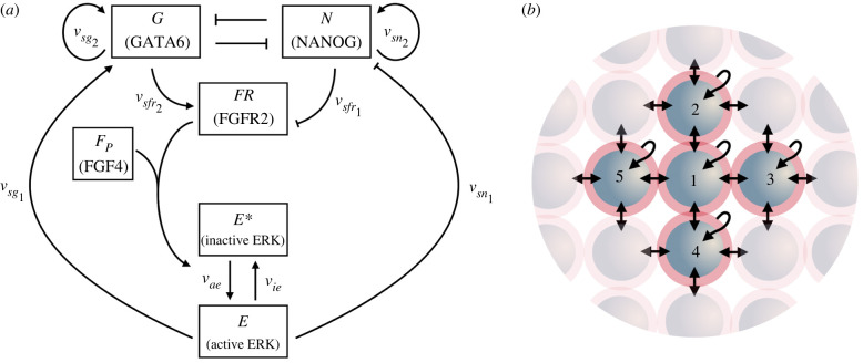
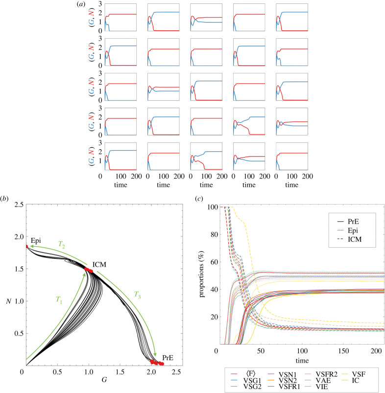
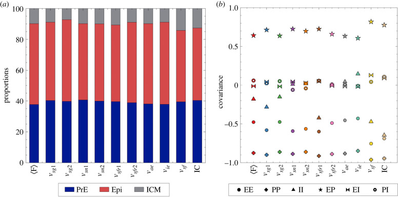
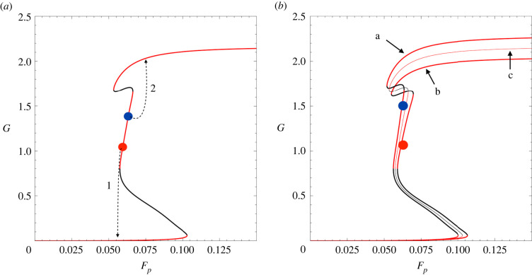
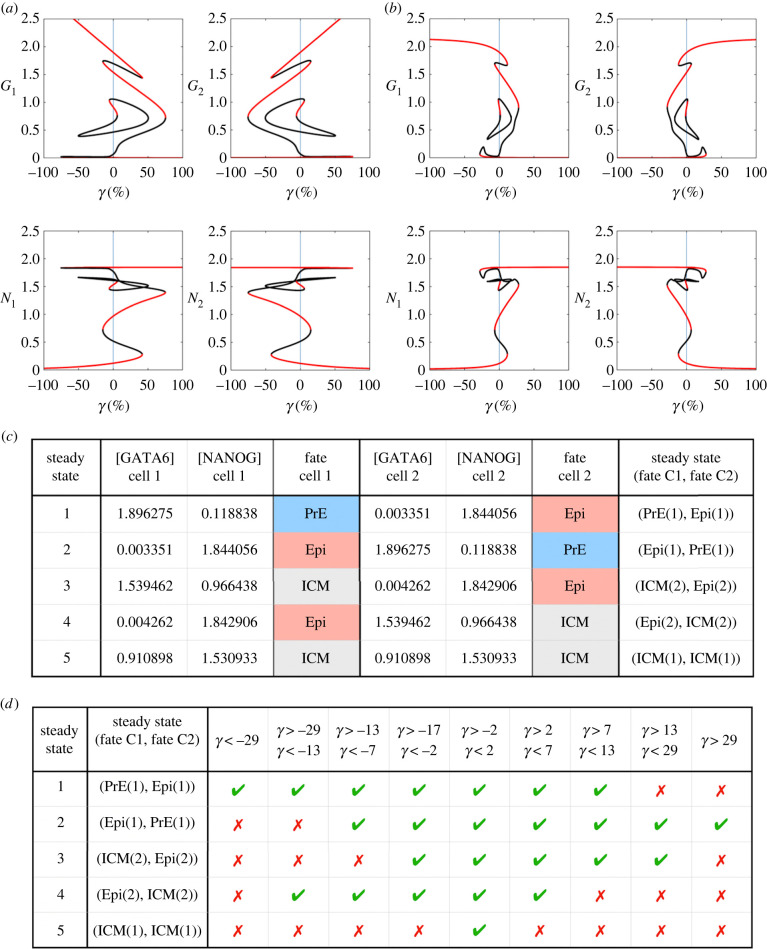
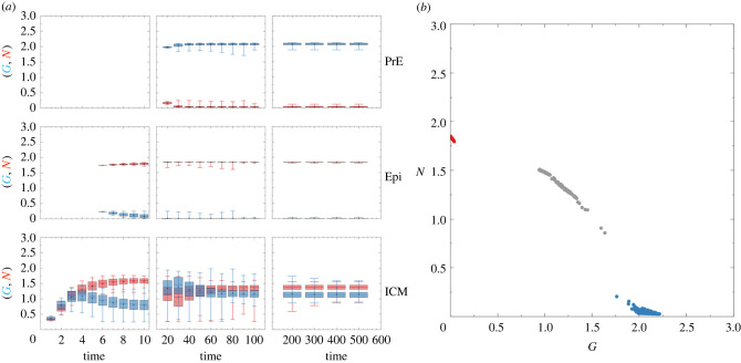
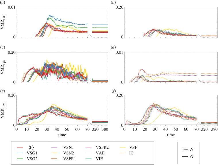
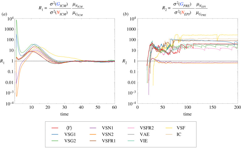
During development, cells from a population of common progenitors evolve towards different fates characterized by distinct levels of specific transcription factors, a process known as cell differentiation. This evolution is governed by gene regulatory networks modulated by intercellular signalling. In order to evolve towards distinct fates, cells forming the population of common progenitors must display some heterogeneity. We applied a modelling approach to obtain insights into the possible sources of cell-to-cell variability initiating the specification of cells of the inner cell mass into epiblast or primitive endoderm cells in early mammalian embryo. At the single-cell level, these cell fates correspond to three possible steady states of the model. A combination of numerical simulations and bifurcation analyses predicts that the behaviour of the model is preserved with respect to the source of variability and that cell-cell coupling induces the emergence of multiple steady states associated with various cell fate configurations, and to a distribution of the levels of expression of key transcription factors. Statistical analysis of these time-dependent distributions reveals differences in the evolutions of the variance-to-mean ratios of key variables of the system, depending on the simulated source of variability, and, by comparison with experimental data, points to the rate of synthesis of the key transcription factor NANOG as a likely initial source of heterogeneity.

Keywords: bifurcation; cell differentiation; noise; probability distribution; tristability; variability.

Figure 1.

(a) Intracellular GRN controlling the specification of ICM cells into Epi and PrE. GATA6 and NANOG inhibit each other and self-activate. FGF/ERK signalling, which is activated through the binding of FGF4 to the receptor FGFR2, activates GATA6 and inhibits NANOG. The synthesis of the receptor FGFR2 is activated by GATA6 and inhibited by NANOG. (b) To simulate the emergence of Epi and PrE cells in a population, we consider a static network of 25 cells, disposed on a 5 × 5 square lattice with periodic boundary conditions. Intercellular signalling is achieved through the secretion of FGF4 in the extracellular medium. Each cell synthesizes and releases FGF4 at a rate proportional to its level of NANOG and senses the (average) level of FGF4 produced by the neighbouring cells and by itself.

Figure 2.

(a) Time evolution of GATA6 (G, blue curves) and NANOG (N, red curves) in each cell from a population of 25 cells obtained when heterogeneity is applied on the synthesis rate of GATA6, v_sg1 (γ_max = 10%). Initial conditions are identical for each cell: G₀ = N₀ = 0, FR₀ = 2.8, ERK₀ = 0.25, F₀ = 0.066. (b) Phase plane trajectories corresponding to the time evolution are shown in (a). Red dots represent the concentration of GATA6 and NANOG at steady state for Epi, PrE and ICM cells. (c) Time evolution of the PrE (straight lines), Epi (dotted lines) and ICM (dashed lines) proportions computed for each parameter on which we applied heterogeneity (shown in different colours). The cell states are assigned as follows: a cell will be considered as ‘Epi’ if N > G and G < 0.3. The reverse criterion is applied for the PrE cells, which are defined by N < G and N < 0.3. Cells that do not satisfy any of these criteria are in the ICM state. These proportions are averaged over 100 simulations.

Figure 3.

(a) Proportions of PrE (blue), Epi (red) and ICM (grey) cells observed at the end of the simulation when variability is applied on each kinetic parameter (with γ_max = 10%), or on initial conditions (IC). In this case, γ_i is introduced in the initial conditions of each variable X (simultaneously): X₀ → X₀ (1 + γ_i) for X = ERK or FR and X₀ → γ_i (with γ_i > 0) for X = N or G, with G(0) = N(0) = 0 and F₀ = 0.066. ERK(0) and FR(0) are the steady state values of these variables corresponding to G(0) = N(0) = 0 and F₀ = 0.066. The state of a cell is defined at the end of the simulation with the same criteria as in figure 2. The proportions are averaged over 100 simulations. (b) Spatial normalized covariance values between Epi cells and Epi cells (EE for ${\tilde{C}}_{\mathrm{Epi}:\mathrm{Epi}}$), PrE cells and PrE cells (PP for ${\tilde{C}}_{\mathrm{PrE}:\mathrm{PrE}}$), ICM cells and ICM cells (II for ${\tilde{C}}_{\mathrm{ICM}:\mathrm{ICM}}$), Epi cells and PrE cells (EP for ${\tilde{C}}_{\mathrm{Epi}:\mathrm{PrE}}$), Epi cells and ICM cells (EI for ${\tilde{C}}_{\mathrm{Epi}:\mathrm{ICM}}$), PrE cells and ICM cells (PI for ${\tilde{C}}_{\mathrm{PrE}:\mathrm{ICM}}$) (see electronic supplementary material, information). These spatial normalized covariance values are calculated at steady state by an average over 100 simulations for which values of γ_i for each cell i are reassigned at each simulation (γ_max = 10%).

Figure 4.

(a) Bifurcation diagram of the one-cell model showing the Gata6 concentration at steady state as a function of F_P. (b) Bifurcation diagrams obtained for different values of v_sg1. For curve a, v_sg1 is slightly decreased (v_sg1 → v_sg1 − 10%) and for curve b, v_sg1 is slightly increased (v_sg1 → v_sg1 + 10%.). Curve ‘c’ corresponds to the absence of variability (same as in (a)). Red curves represent the stable branches, whereas black curves represent the unstable branches. Red and blue dots schematically represent 2 cells differing by their sensitivity to FGF4 (a) or by their v_sg1 value (b). In both cases, starting from the same initial conditions (with N = G = 0), the two cells first evolve towards the ICM state. Then, due to an initial decrease of F_p, the red cell specifies into Epi (while the blue cells remain on the ICM branch). Later, following an increase of F_p, the blue cell specifies into PrE (see explanation in the text).

Figure 5.

Bifurcation diagrams of the two-cell model with variability on (a) F_P and (b) v_sg1. Red and black lines represent stable and unstable branches, respectively. The x-axis indicates the variability γ applied on the corresponding parameter. The y-axis indicates the GATA6 or NANOG stationary concentration values for each cell. (c) List of possible steady states (and corresponding combinations of cell fates) for the coupled two-cell system when there is no variability in the system (γ = 0). (d) Domains of existence each steady state as a function of γ for the coupled two-cell system when variability is applied on F_P. Each column represents a range of values of γ (in %, rounded) in which a given combination of cell fates is possible (green tick) or not (red cross) for the system.

Figure 6.

(a) Time evolution of the distribution of the NANOG (red) and GATA6 (blue) concentrations when heterogeneity is applied on the v_sg1 parameter (γ_max =10%). The distributions are represented by box plots where the boxed region represents 50% of the values of the distribution, black dots the average values, the bold colour line the median and the extremities represent the maximum/minimum value. The state of a cell is defined with the same criteria as in figure 2 for every time unit from t = 0 to t = 10, (left panels), for every 10-time units from t = 20 to t = 100, (middle panels) and for every 100-time units from t = 200 to t = 500, (right panels). The height of each box plot can be interpreted as the variance of the distribution. Statistics were performed on the concentrations in the 25 cells over 100 simulations. (b) Stationary values of the concentration in 25 cells over 100 simulations are represented in a phase plane when heterogeneity is applied on v_sg1 parameter. Grey dots correspond to cells in the ICM state, red dots denote the cells in the Epi state and blue dots denote the cells in the PrE state.

Figure 7.

Time evolution of the VMR of the GATA6 (straight lines, (a,c,e)) and NANOG (dotted lines, (b,d,f)), computed for each parameter on which we applied heterogeneity (shown in different colours). Statistics were performed on the concentrations of these two factors for 25 cells over 100 simulations (γ_max = 10%). The first 70 time units show all the different specification phases and the 100 last time units show that the concentrations (and therefore the VMRs) do not change at steady state. The cells states are assigned as in figure 2.

Figure 8.

Time evolution of the ratio R between VMR of the GATA6 concentrations and NANOG concentrations (a) in the ICM cells and (b) in the PrE and Epi cells, respectively. The ratio was computed for each parameter on which heterogeneity is applied (represented in different colours). Statistics were performed on the concentrations of the 25 cells over 100 simulations (γ_max = 10%).

References

1. Zhou JX, Huang S. 2011. Understanding gene circuits at cell-fate branch points for rational cell reprogramming. Trends Genet. 27, 55-62. (10.1016/j.tig.2010.11.002) - DOI - PubMed
1. De Caluwé J, Tosenberger A, Gonze D, Dupont G. 2019. Signalling-modulated gene regulatory networks in early mammalian development. J. Theor. Biol. 463, 56-66. (10.1016/j.jtbi.2018.12.008) - DOI - PubMed
1. Eldar A, Elowitz M. 2010. Functional roles for noise in genetic circuits. Nature 467, 167-173. (10.1038/nature09326) - DOI - PMC - PubMed
1. Torres-Padilla ME, Chambers I. 2014. Transcription factor heterogeneitiy in pluripotent stem cells: a stochastic advantage. Development 141, 2173-2181. (10.1242/dev.102624) - DOI - PubMed
1. Graham SJ, Zernicka-Goetz M. 2016. The acquisition of cell fate in mouse development: how do cells first become heterogeneous? Curr. Top. Dev. Biol. 117, 671-695. (10.1016/bs.ctdb.2015.11.021) - DOI - PubMed