. 2022 Jul 22;7(1):65.
doi: 10.1186/s41235-022-00397-3.

Toward a more comprehensive modeling of sequential lineups

Affiliations

Toward a more comprehensive modeling of sequential lineups

David Kellen et al. Cogn Res Princ Implic. .

Abstract

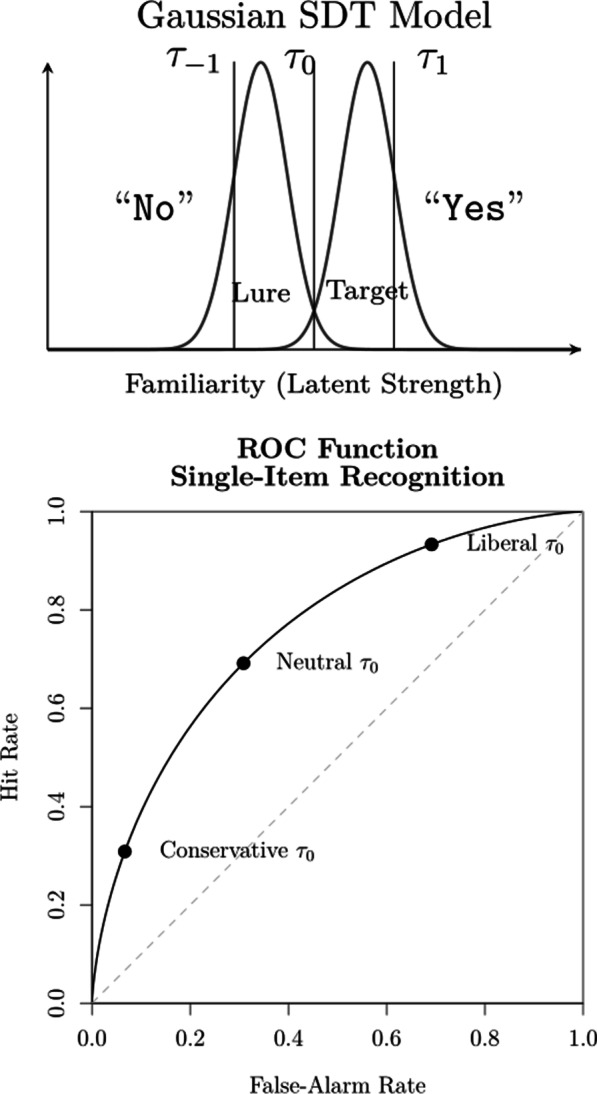
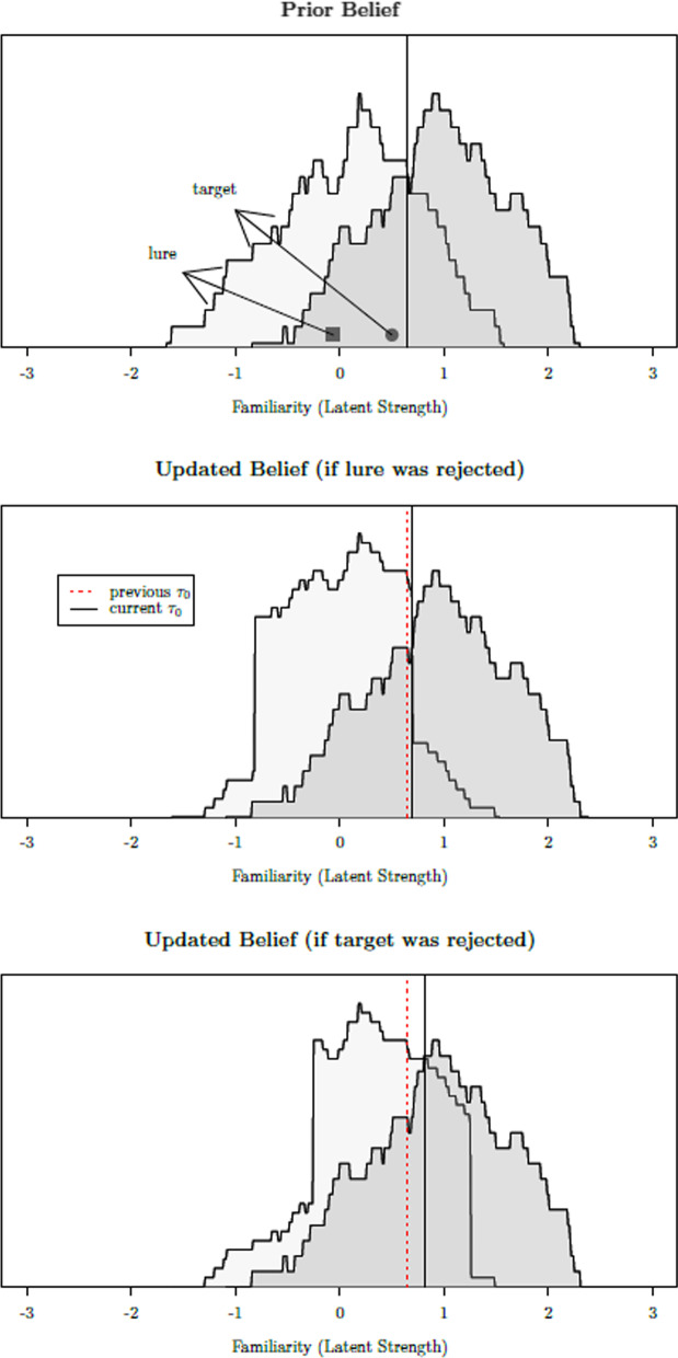
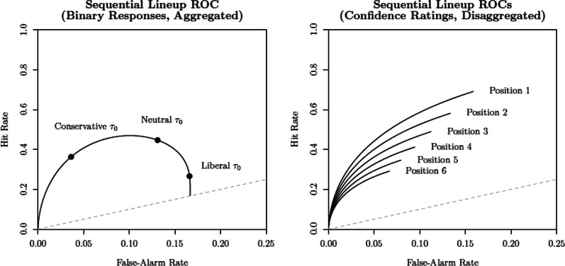
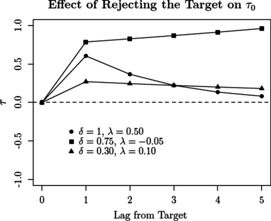
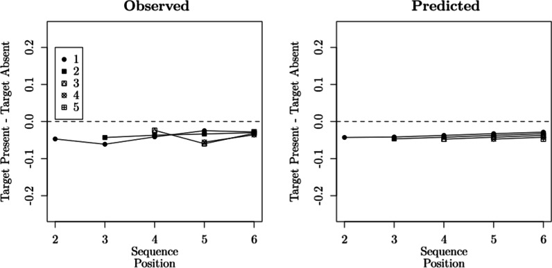
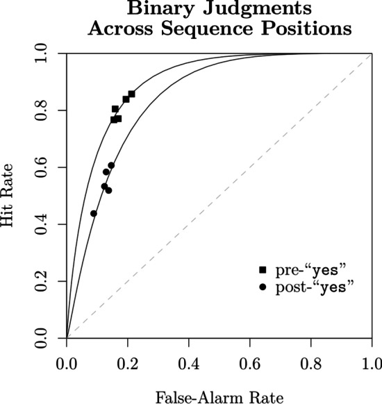
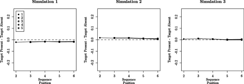
Sequential lineups are one of the most commonly used procedures in police departments across the USA. Although this procedure has been the target of much experimental research, there has been comparatively little work formally modeling it, especially the sequential nature of the judgments that it elicits. There are also important gaps in our understanding of how informative different types of judgments can be (binary responses vs. confidence ratings), and the severity of the inferential risks incurred when relying on different aggregate data structures. Couched in a signal detection theory (SDT) framework, the present work directly addresses these issues through a reanalysis of previously published data alongside model simulations. Model comparison results show that SDT modeling can provide elegant characterizations of extant data, despite some discrepancies across studies, which we attempt to address. Additional analyses compare the merits of sequential lineups (with and without a stopping rule) relative to showups and delineate the conditions in which distinct modeling approaches can be informative. Finally, we identify critical issues with the removal of the stopping rule from sequential lineups as an approach to capture within-subject differences and sidestep the risk of aggregation biases.


Conflict of interest statement

The authors declare no competing interests.

Figures

Fig. 1
Fig. 1
Top panel: Illustration of the Gaussian SDT model. The vertical lines represent the response criterion τ0 and the confidence criteria τ-1 and τ1. Bottom panel: Example of a ROC function for the case of single-item recognition
Fig. 2
Fig. 2
Top panel: The believed distribution of latent strength values for targets (darker gray) and lures (lighter gray) up to the point in which the target (solid circle) or a lure (solid square) are encountered. Note that both latent strengths are below the response criterion (solid black line), which is set at the point of equal likelihood (i.e., where both distributions intersect). Middle panel: The updated believed distributions of latent strength values if the lure was encountered and rejected. Bottom panel: The updated believed distributions of latent strength values if the target was encountered and rejected instead. In both the middle and bottom panels, the prior response criterion (dotted red line) is given for reference
Fig. 3
Fig. 3
Example of ROCs obtained in a sequential lineup procedure. Left panel: The predicted ROC function when varying response criterion τ0 and aggregating across sequence positions. Right panel: Confidence rating ROCs obtained for each sequence position
Fig. 4
Fig. 4
Effect of previously encountering and rejecting the target on τ0, as a function of parameters δ and λ. Lag=0 denotes the value of τ when the target is encountered
Fig. 5
Fig. 5
Illustration of how the latent strength distributions can change across sequence positions under different SDT models. The dashed lines indicate the origin of the latent strength scale
Fig. 6
Fig. 6
Left panel: Comparison of model predictions (SDTτ4,) and the data. Right panel: Comparison of model predictions coming from the SDTτ2, and SDTτ4, models
Fig. 7
Fig. 7
Differences in the conditional probability of responding “yes” to a lure in sequence position i between target-present lineups (in which the target was previously rejected) and target-absent lineups. The different symbols/lines distinguish the preceding position taken by the target in target-present lineups (reanalysis of Wilson et al., 2019)
Fig. 8
Fig. 8
Examples of the effect of previously encountering and rejecting the target on ordered confidence criteria τi, which is established as a function of parameters ω, γ, and η and Lag =i-h. Lag=0 denotes the value of the criteria when the target is encountered. For illustrative purposes, τ0 remains fixed at 0 across lags and the contiguous confidence criteria in Lag=0 are equidistant
Fig. 9
Fig. 9
Observed confidence rating ROCs and the corresponding predictions from SDTτ4, (Reanalysis of Wilson et al., 2019)
Fig. 10
Fig. 10
Distribution of ΔG2 values, obtained from the comparison of the SDTτ4, and SDTτ4,μ1 models, when generating the confidence rating data from the latter under different values of α2-6. Two-hundred datasets were generated per scenario. The black circle corresponds to the ΔG2=0.01 observed with the real data (see Table 3). The red lines correspond to polynomial spline approximations of the ΔG2 distributions. Please note that the ranges of both axes vary across panels
Fig. 11
Fig. 11
True and estimated da from the SDTτ4, model, under different n per lineup condition
Fig. 12
Fig. 12
Confidence rating ROCs (from Wilson et al., 2019) obtained in position 1 of the sequential lineup procedure and the showup procedure
Fig. 13
Fig. 13
Expected utilities associated with different procedures, as a function of the probability that the suspect is guilty (Pguilty) and the outcome frequencies reported in Table 5. SR = stopping rule. The gray dashed line corresponds to the Pguilty estimate reported by Wixted et al. (2016)
Fig. 14
Fig. 14
Observed confidence rating ROCs and the corresponding predictions from SDTτ4,μ1 (Reanalysis of Dunn et al., 2022)
Fig. 15
Fig. 15
Differences in the conditional probability of responding “yes” in sequence position i between target-present and target-absent lineups. The different symbols distinguish the preceding position taken by the target in target-present lineups
Fig. 16
Fig. 16
Binary response ROCs (from Wilson et al., 2019) obtained with marginal responses per sequence position (each point corresponds to a sequence position, from 2 to 6). Black squares denote cases in which no “yes” responses were made in any previous positions (pre-“yes”). Black circles denote the complementary cases in at least one “yes” response was previously made (post-“yes”)
Fig. 17
Fig. 17
Simulated differences in the conditional probability of responding “yes” in sequence position i between target-present and target-absent lineups. The different symbols distinguish the preceding position taken by the target in target-present lineups

Similar articles

References

    1. Barr DJ, Levy R, Scheepers C, Tily HJ. Random effects structure for confirmatory hypothesis testing: Keep it maximal. Journal of memory and language. 2013;68:255–278. doi: 10.1016/j.jml.2012.11.001. - DOI - PMC - PubMed
    1. Batchelder WH, Riefer DM. Multinomial processing models of source monitoring. Psychological Review. 1990;97:548–564. doi: 10.1037/0033-295X.97.4.548. - DOI
    1. Baumann C, Singmann H, Gershman SJ, von Helversen B. A linear threshold model for optimal stopping behavior. Proceedings of the National Academy of Sciences. 2020;117:12750–12755. doi: 10.1073/pnas.2002312117. - DOI - PMC - PubMed
    1. Birnbaum MH. Testing mixture models of transitive preference: Comment on Regenwetter, Dana, and Davis-Stober (2011) Psychological Review. 2011;118:675–683. doi: 10.1037/a0023852. - DOI - PubMed
    1. Birnbaum MH. True-and-error models violate independence and yet they are testable. Judgment and Decision making. 2013;8:717–737.

Publication types

LinkOut - more resources