. 2022 Jul 21;157(3):034106.
doi: 10.1063/5.0087058.

Computing transition path theory quantities with trajectory stratification

Affiliations

Computing transition path theory quantities with trajectory stratification

Bodhi P Vani et al. J Chem Phys. .

Abstract

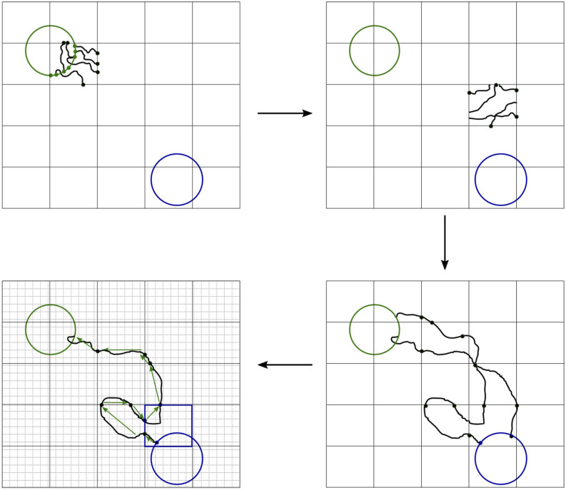
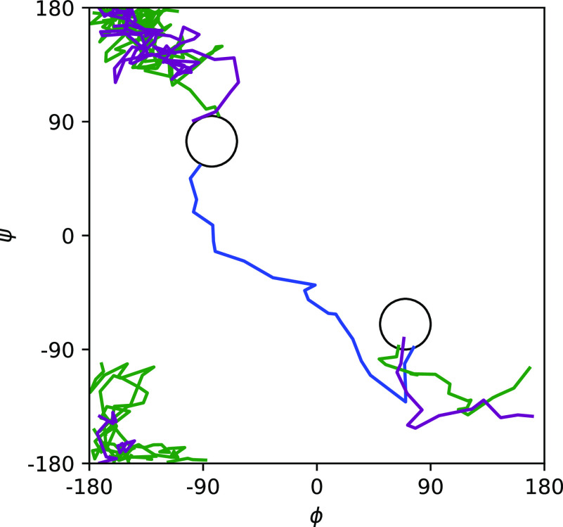
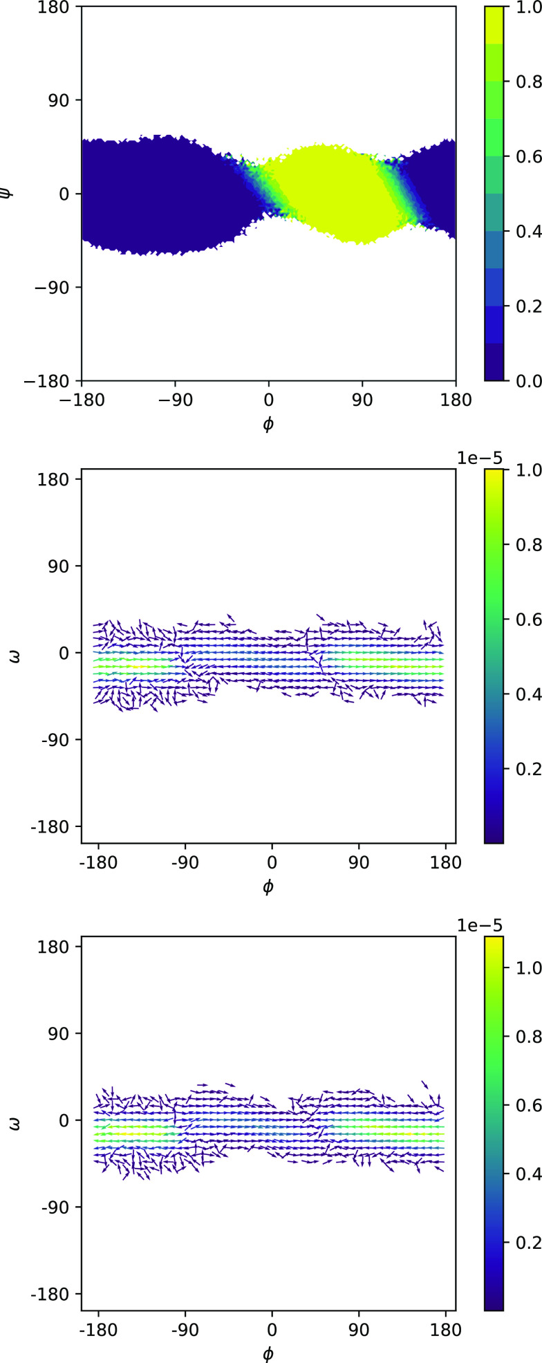
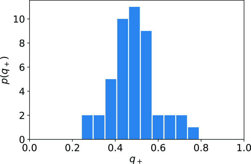
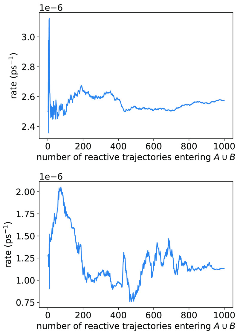
Transition path theory computes statistics from ensembles of reactive trajectories. A common strategy for sampling reactive trajectories is to control the branching and pruning of trajectories so as to enhance the sampling of low probability segments. However, it can be challenging to apply transition path theory to data from such methods because determining whether configurations and trajectory segments are part of reactive trajectories requires looking backward and forward in time. Here, we show how this issue can be overcome efficiently by introducing simple data structures. We illustrate the approach in the context of nonequilibrium umbrella sampling, but the strategy is general and can be used to obtain transition path theory statistics from other methods that sample segments of unbiased trajectories.


Figures

FIG. 1.
FIG. 1.
Schematic of the algorithm. (upper left) Define the metastable states and the strata (black grid) and initialize the data structures (step 1). In the example shown, trajectories are initialized from the upper left metastable state boundary, so the last metastable state visited is known. (upper right) In each stratum, draw configurations from γij(dx), save pointers to the associated γij(dx) elements, and then run unbiased dynamics from these configurations until the trajectories exit the stratum (steps 2b and 2c). A single example stratum is shown. (lower right) As the simulation progresses, each point in γij(dx) may give rise to segments of reactive or unreactive trajectories. Save the collective variable values associated with these trajectory segments (step 2d). (lower left) When a reactive or unreactive trajectory is realized (i.e., a trajectory segment enters a metastable state), trace back from pointer to pointer to determine the sequences of strata and collective variable grid sites (gray grid) visited (step 3). Use these to increment unnormalized statistics with appropriate weights (steps 3a–3c). Note that the collective variable grid sites and the strata need not coincide.
FIG. 2.
FIG. 2.
Alanine dipeptide with the three dihedral angles labeled: ϕ [C5–N7–C9(α)–C15], ψ [N7–C9(α)–C15–N17], and ω [C1–C5–N7–C9(α)]. Colors are cyan for carbon, blue for nitrogen, white for hydrogen, and red for oxygen.
FIG. 3.
FIG. 3.
Potentials of mean force computed from the NEUS simulations: projections on (top) ϕ and ψ and (bottom) ϕ and ω. The stable states are marked with white circles on the top plot.
FIG. 4.
FIG. 4.
Committor (top) and forward (middle) and backward (bottom) reactive currents for the C7ax → C7eq transition of the alanine dipeptide, plotted on the ϕψ-plane.
FIG. 5.
FIG. 5.
Example trajectories plotted on the ϕψ-plane. The circles mark the metastable states.
FIG. 6.
FIG. 6.
Committor (top) and forward (middle) and backward (bottom) reactive currents for the C7ax → C7eq transition of the alanine dipeptide, plotted on the ϕω-plane. For the reactive currents, only grid points with data from at least five trajectories are shown.
FIG. 7.
FIG. 7.
Histogram of committors computed by shooting for 137 structures predicted to have 0.49<q+θ<0.51 for the reaction from A to B. 20 independent simulations were used for each configuration.
FIG. 8.
FIG. 8.
Rates computed directly from the flux into B (top) and by integrating the reactive currents (bottom). An equal number of crossings between metastable states each way is used for each point on the horizontal axis.

Similar articles

Cited by

References

    1. Ma A. and Dinner A. R., “Automatic method for identifying reaction coordinates in complex systems,” J. Phys. Chem. B 109, 6769–6779 (2005).10.1021/jp045546c - DOI - PubMed
    1. Vanden-Eijnden E., “Transition path theory,” in Computer Simulations in Condensed Matter Systems: From Materials to Chemical Biology Volume 1, edited by Ferrario M., Ciccotti G., and Binder K. (Springer Berlin Heidelberg, Berlin, Heidelberg, 2006), pp. 453–493.
    1. E W. and Vanden-Eijnden E., “Towards a theory of transition paths,” J. Stat. Phys. 123, 503 (2006).10.1007/s10955-005-9003-9 - DOI
    1. Metzner P., Schütte C., and Vanden-Eijnden E., “Illustration of transition path theory on a collection of simple examples,” J. Chem. Phys. 125, 084110 (2006).10.1063/1.2335447 - DOI - PubMed
    1. Noé F., Schütte C., Vanden-Eijnden E., Reich L., and Weikl T. R., “Constructing the equilibrium ensemble of folding pathways from short off-equilibrium simulations,” Proc. Natl. Acad. Sci. U. S. A. 106, 19011–19016 (2009).10.1073/pnas.0905466106 - DOI - PMC - PubMed