Alluvial connectivity in multi-channel networks in rivers and estuaries

Abstract

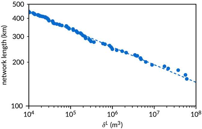
Channels in rivers and estuaries are the main paths of fluvial and tidal currents that transport sediment through the system. While network representations of multi-channel systems and their connectivity are quite useful for characterisation of braiding patterns and dynamics, the recognition of channels and their properties is complicated because of the large bed elevation variations, such as shallow shoals and bed steps that render channels visually disconnected. We present and analyse two mathematically rigorous methods to identify channel networks from a terrain model of the river bed. Both methods construct a dense network of locally steepest-descent channels from saddle points on the terrain, and select a subset of channels with a certain minimum sediment volume between them. This is closely linked to the main mechanism of channel formation and change by displacement of sediment volume. The two methods differ in how they compute these sediment volumes: either globally through the entire length of the river, or locally. We compare the methods for the measured bathymetry of the Western Scheldt estuary, The Netherlands, over the past decades. The global method is overly sensitive to small changes elsewhere in the network compared to the local method. We conclude that the local method works best conceptually and for stability reasons. The associated concept of alluvial connectivity between channels in a network is thus the inverse of the volume of sediment that must be displaced to merge the channels. Our method opens up possibilities for new analyses as shown in two examples. First, it shows a clear pattern of scale dependence on volume of the total network length and of the number of nodes by a power law relation, showing that the smaller channels are relatively much shorter. Second, channel bifurcations were found to be predominantly mildly asymmetrical, which is unexpected from fluvial bifurcation theory.

Keywords: algorithms; bifurcation; connectivity; estuary; network.

FIGURE 1

Whitehaven estuary (Australia, 20° 16 ^′ S, 149° 1 ^′ E). Both images show channel segments and dead‐ended channels disconnected from the network by shoals and bars. The 2013 image was taken at a slightly lower water surface elevation than the 2016 image. Image source: Google Earth, accessed March 2021 [Color figure can be viewed at wileyonlinelibrary.com]

FIGURE 2

Sketch of a river‐bed DEM (a), minima and saddle points (b), and the Morse–Smale complex, with the Morse–Smale edges in dark blue and the Morse–Smale cells coloured (c) [Color figure can be viewed at wileyonlinelibrary.com]

FIGURE 3

Steps in the striation method: (a) select a Morse–Smale cell (here marked with a cross) and compute the two lowest paths around it; (b) repeat this procedure until all Morse–Smale cells have been used; (c) select paths with volume at least δ _G between them (shown here for three values of δ _G ); (d) post‐process the selected paths into a network (figure adapted from Hiatt et al., 2020) [Color figure can be viewed at wileyonlinelibrary.com]

FIGURE 4

Steps in the volume persistence algorithm: repeatedly select a saddle in the Morse–Smale complex (a), and if the volume of sediment around the saddle is lower than the threshold remove the saddle to merge the adjacent Morse–Smale cells. After processing all saddles, the final network remains (b). (c,d) Two examples of computing volumes around saddles (the red‐shaded area indicates the measured volume) [Color figure can be viewed at wileyonlinelibrary.com]

FIGURE 5

Definition and examples of bifurcation angle asymmetry [Color figure can be viewed at wileyonlinelibrary.com]

FIGURE 6

Map of the bathymetry in 2013 (a), two networks created by the striation method with different thresholds for the sand volume δ _G (b), the network by the persistence method where links are colour coded by sand volume δ _L (c), and a sliced morphology map taken at elevation 0 m AMSL (d) [Color figure can be viewed at wileyonlinelibrary.com]

FIGURE 7

Comparison of the number of corresponding channel positions in four volume classes applicable to the striation method (horizontal, ${\delta }_G=10^6,10^7,10^8,10^9$ m³) and persistence method (vertical, ${\delta }_L=10^4,10^5,10^6,10^7$ m³)

FIGURE 8

Maps of the flow velocity in cm/s in 2013 for ebb (a) and flood (b), and the networks as created by the persistence method for ebb (c) and flood (d) [Color figure can be viewed at wileyonlinelibrary.com]

FIGURE 9

Measures of the whole network. (a) Total length of all network links through time. (b) Number of nodes in the network. Red: striation method, from top to bottom for ${\delta }_G=10^6,10^7,10^8,10^9$ m³. Blue: persistence method, from top to bottom for ${\delta }_L=10^4,10^5,10^6,10^7$ m³ [Color figure can be viewed at wileyonlinelibrary.com]

FIGURE 10

Network scaling for the persistence method applied to the 2013 bathymetry [Color figure can be viewed at wileyonlinelibrary.com]

FIGURE 11

Asymmetry of channel bifurcations calculated from all persistence networks through time, subdivided between bifurcations in the general ebb direction and in the general flood direction, and between large side channels and small connecting channels. (a) Distribution of vertical bifurcation asymmetry: bed elevation differences between the bifurcate normalised with bed elevation (m AMSL) in the upstream channel. (b) Distribution of horizontal bifurcation asymmetry: difference in bifurcate angles with the upstream channel normalised with the sum of the angles. (c–f) Comparison of horizontal and asymmetry for four categories of bifurcations [Color figure can be viewed at wileyonlinelibrary.com]

References

1. Agarwal, P. , de Berg, M. , Bose, P. , Dobrint, K. , van Kreveld, M. , Overmars, M. et al. (1996) The complexity of rivers in triangulated terrains, Proceedings of the 8th Canadian Conference on Computational Geometry (CCCG).
1. Arge, L. , Chase, J.S. , Halpin, P. , Toma, L. , Vitter, J.S. , Urban, D. et al. (2003) Efficient flow computation on massive grid terrain datasets. GeoInformatica, 7(4), 283–313. 10.1023/A:1025526421410 - DOI
1. Ashmore, P. (1991) Channel morphology and bed load pulses in braided, gravel‐bed streams. Geografiska Annaler: Series a, Physical Geography, 73(1), 37–52. 10.1080/04353676.1991.11880331 - DOI
1. Baar, A.W. , Boechat Albernaz, M. , van Dijk, W.M. & Kleinhans, M.G. (2019) Critical dependence of morphodynamic models of fluvial and tidal systems on empirical downslope sediment transport. Nature Communications, 10(1), 4903. 10.1038/s41467-019-12753-x - DOI - PMC - PubMed
1. Bertoldi, W. , Zanoni, L. & Tubino, M. (2009) Planform dynamics of braided streams. Earth Surface Processes and Landforms, 34(4), 547–557. 10.1002/esp.1755 - DOI