Population-based sequencing of Mycobacterium tuberculosis reveals how current population dynamics are shaped by past epidemics

Abstract

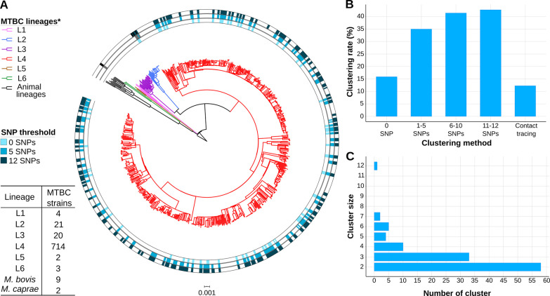
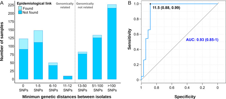
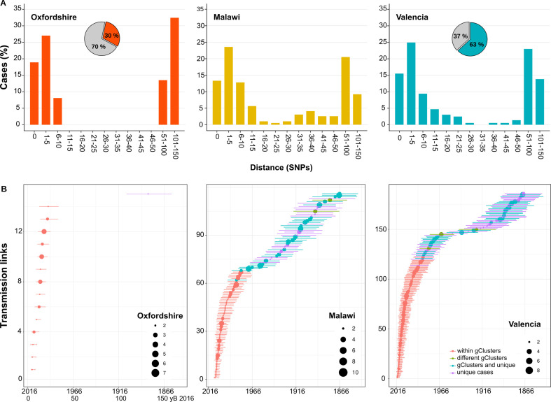
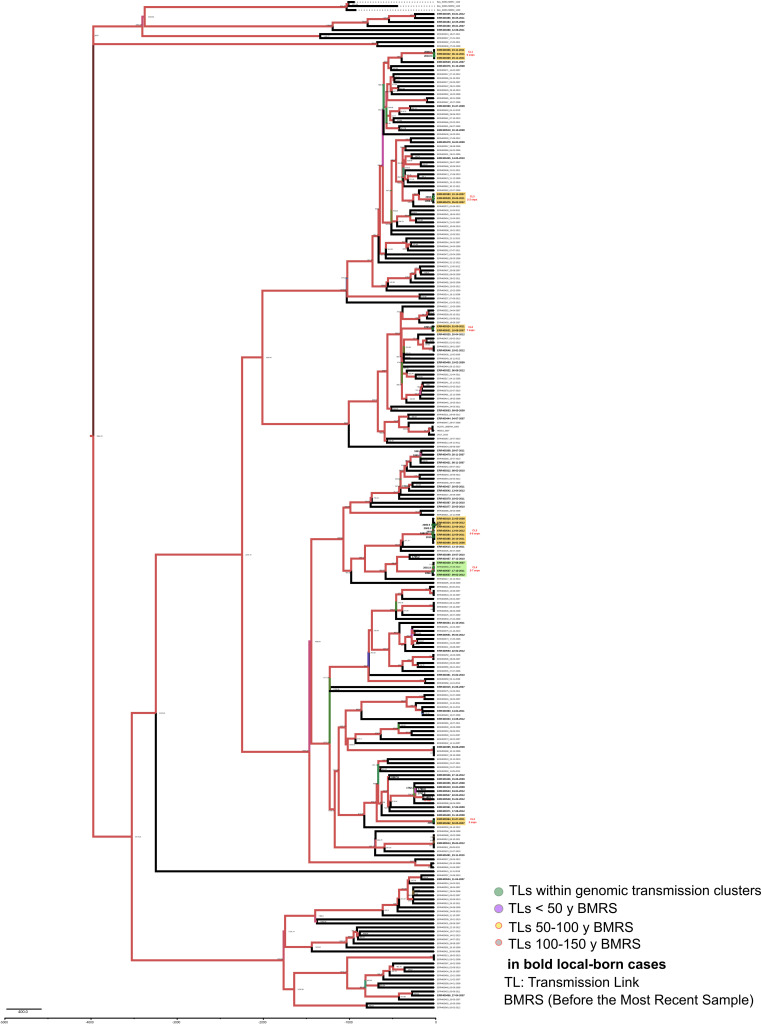
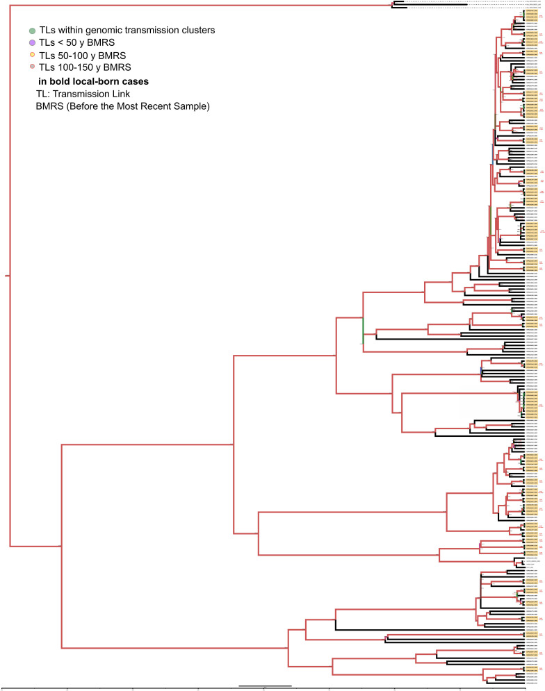
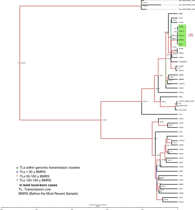
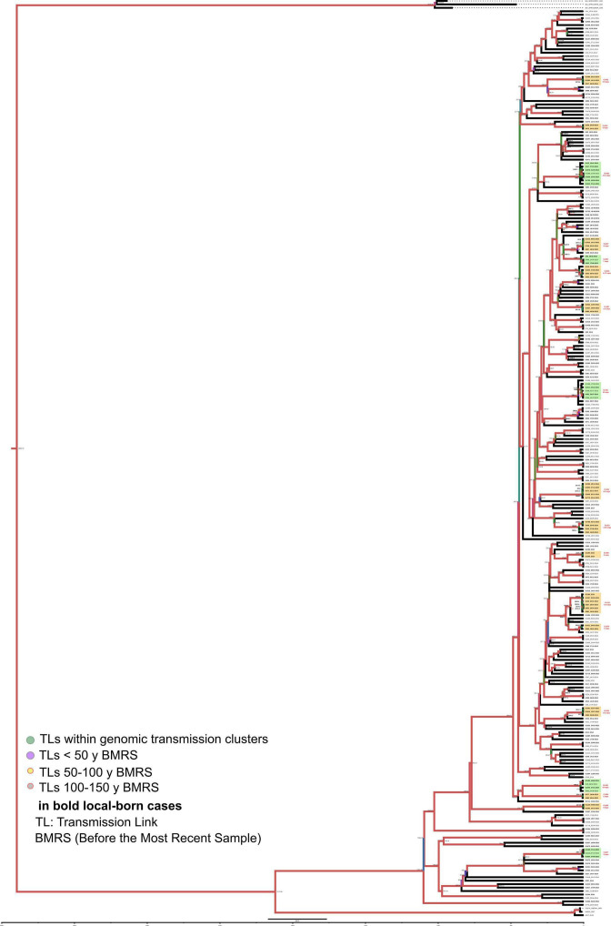
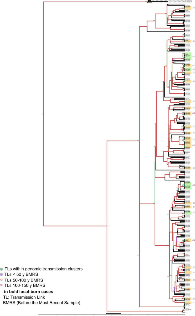
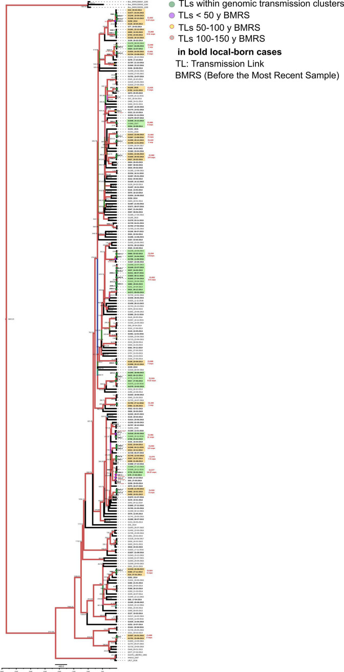
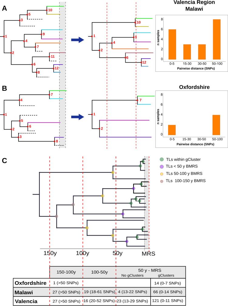
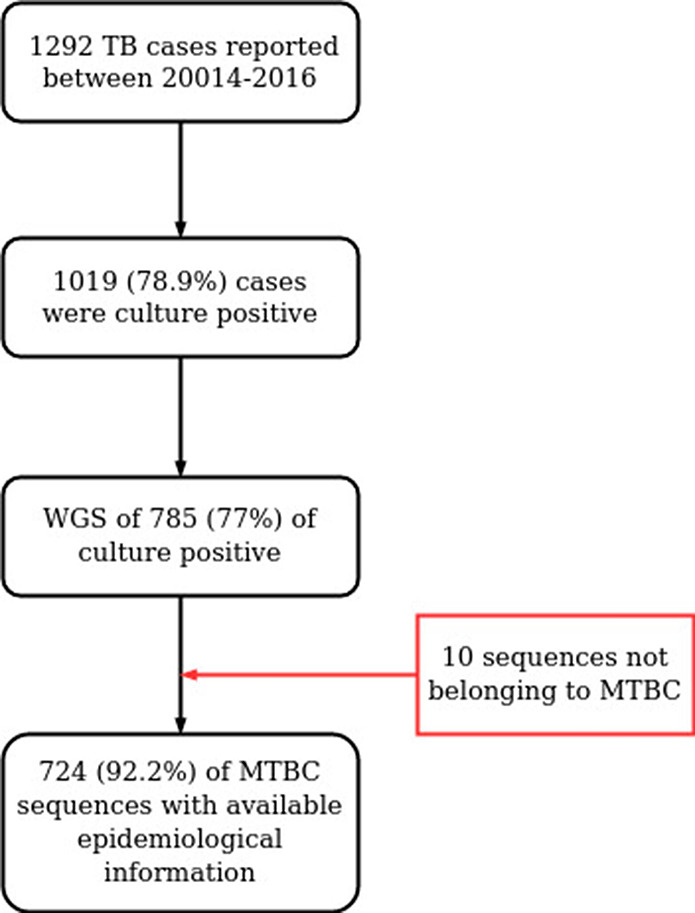
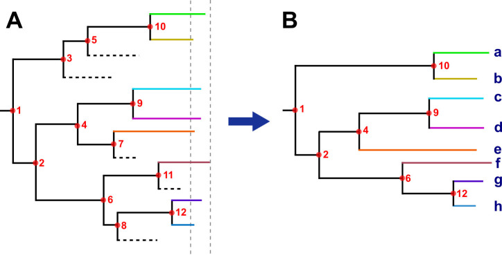
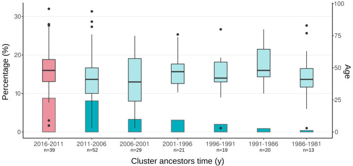
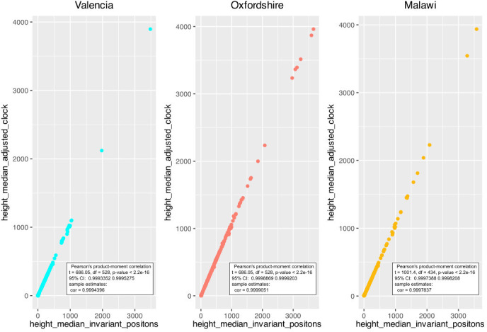
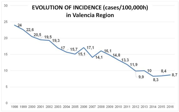
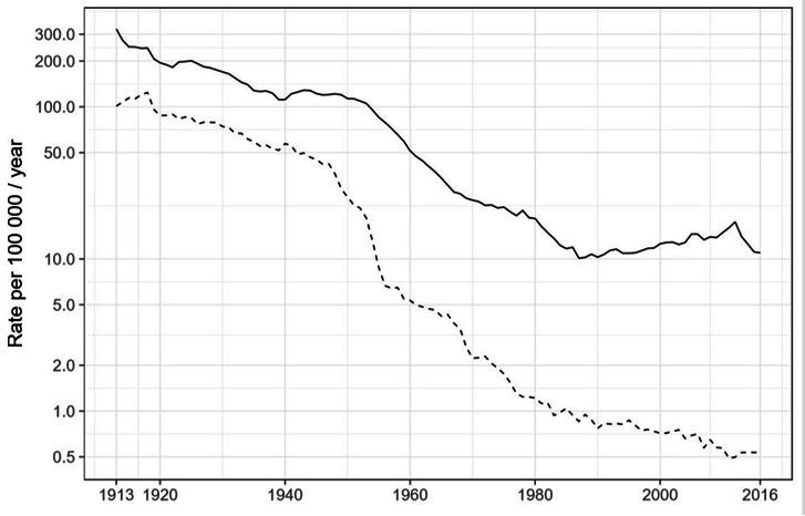
Transmission is a driver of tuberculosis (TB) epidemics in high-burden regions, with assumed negligible impact in low-burden areas. However, we still lack a full characterization of transmission dynamics in settings with similar and different burdens. Genomic epidemiology can greatly help to quantify transmission, but the lack of whole genome sequencing population-based studies has hampered its application. Here, we generate a population-based dataset from Valencia region and compare it with available datasets from different TB-burden settings to reveal transmission dynamics heterogeneity and its public health implications. We sequenced the whole genome of 785 Mycobacterium tuberculosis strains and linked genomes to patient epidemiological data. We use a pairwise distance clustering approach and phylodynamic methods to characterize transmission events over the last 150 years, in different TB-burden regions. Our results underscore significant differences in transmission between low-burden TB settings, i.e., clustering in Valencia region is higher (47.4%) than in Oxfordshire (27%), and similar to a high-burden area as Malawi (49.8%). By modeling times of the transmission links, we observed that settings with high transmission rate are associated with decades of uninterrupted transmission, irrespective of burden. Together, our results reveal that burden and transmission are not necessarily linked due to the role of past epidemics in the ongoing TB incidence, and highlight the need for in-depth characterization of transmission dynamics and specifically tailored TB control strategies.

Keywords: Mycobacterium tuberculosis; epidemiology; genomic epidemiology; global health; transmission; tuberculosis; whole-genome sequencing.

Figure 1.. Genomic characterization of the study region.

(A) Phylogeny of 775 tuberculosis (TB) isolates collected during the years 2014 and 2016. Each ring represents genomic clusters detected by different single nucleotide polymorphism (SNP) thresholds (0, 5, and 12 SNPs). Mycobacterium canneti was used as an outgroup. (B) Clustering percentage, i.e. percentage of samples within clusters for different SNP thresholds. (C) Number of genomic clusters by different cluster sizes. A 12 SNP threshold was used as a standard. Cluster sizes of 8–11 samples were not detected. *Nomenclature proposed by Comas et al., 2013.

Figure 2.. Comparison between epidemiological and genomic clustering.

(A) Clustered samples using different pairwise distance thresholds, bars denote the number of cases within clusters for each single nucleotide polymorphism (SNP) threshold. Gray dashed line separates the genomically linked samples (clustered) from those unlinked. (B) ROC (Receiver Operating Characteristics) curve for different pairwise distance thresholds between 0 and 2000 SNPs, indicating the optimal SNP cut-off values with its correspondent specificity and sensitivity values, the area under the curve (AUC), and its confidence intervals.

Figure 3.. Historical transmission dynamics analysis.

(A) Distribution of local-born cases clustered by different pairwise distance SNP thresholds. Cases are expressed as the percentage of the plotted samples. Pie charts represent the proportion of local-born (color) and foreign-born (gray) cases in each dataset. (B) Age of local transmission links over time in each setting. Circles represent median time, and lines represent 95% high probability density for each transmission link counted. Circle size represents the number of samples included in the corresponding link. Red denotes those transmission links including only samples within the same genomic transmission clusters (gClusters), green denotes links involving samples from different gClusters, blue denotes samples within gClusters and unique, and purple denotes unique cases. All links were obtained from Figure 3—figure supplements 1–6 and are summarized in Figure 3—source data 1–6.

Figure 3—figure supplement 1.. Bayesian time tree for Oxfordshire dataset.

Sample names in bold represent local born cases. Local clusters (CLs) are highlighted in orange and mixed CLs in green (those including foreign cases). The CL numbers are crossreferenced in Figure 3—source data 1. The transmission links’ (TLs’) dates used in the analysis are indicated in bold and expressed as AD, the other TLs’ dates are indicated as years before 2016 AD. Branch colors represent Bayesian posterior values being red the highest posterior, blue median, and green the lowest values. Numbers in TLs nodes are crossreferenced in Figure 3—source data 4.

Figure 3—figure supplement 2.. Bayesian time tree for Malawi dataset.

Sample names in bold represent local born cases. Local clusters (CLs) are highlighted in orange and mixed CLs in green (those including foreign cases). The CL numbers are crossreferenced in Figure 3—source data 2. The transmission links’ (TLs’) dates used in the analysis are indicated in bold and expressed as AD, the other TLs’ dates are indicated as years before 2016 AD. Branch colors represent Bayesian posterior values being red the highest posterior, blue median, and green the lowest values. Numbers in TLs nodes are crossreferenced in Figure 3—source data 5.

Figure 3—figure supplement 3.. Bayesian time tree for Valencia region dataset.

Sample names in bold represent local born cases. Local clusters (CL) are highlighted in orange and mixed CL in green (those including foreign cases). The CL numbers are crossreferenced in Figure 3—source data 3. The transmission links’ (TLs’) dates used in the analysis are indicated in bold and expressed as AD, the other TLs’ dates are indicated as years before 2016 AD. Branch colors represent Bayesian posterior values being red the highest posterior, blue median and green the lowest values. Numbers in TLs nodes are crossreferenced in Figure 3—source data 6.

Figure 3—figure supplement 4.. Bayesian time tree for Velncia Region dataset.

Sample names in bold represent local born cases. Local clusters are highlighted in orange and mixed clusters in green (those including foreign cases). CL numbers are crossreferencied in Figure 3—source data 3. TLs’ dates used in the analysis are indicated in bold and expressed as AD, the other TLs’ dates are indicated as years before 2016 AD. Branch colors represent bayesian posterior values being red the highest posterior, blue median and green the lowest values. Numbers in TLs nodes are cross referencend in Figure 3—source data 6.

Figure 3—figure supplement 5.. Bayesian time tree for Valencia Region dataset.

Sample names in bold represent local born cases. Local clusters are highlighted in orange and mixed clusters in green (those including foreign cases). CL numbers are crossreferencied in Figure 3—source data 3. TLs’ dates used in the analysis are indicated in bold and expressed as AD, the other TLs’ dates are indicated as years before 2016 AD. Branch colors represent bayesian posterior values being red the highest posterior, blue median and green the lowest values. Numbers in TLs nodes are crossreferencend in Figure 3—source data 6.

Figure 3—figure supplement 6.. Bayesian time tree for Valencia Region dataset.

Sample names in bold represent local born cases. Local clusters are highlighted in orange and mixed clusters in green (those including foreign cases). CL numbers are crossreferencied in Figure 3-source data 3. TLs’ dates used in the analysis are indicated in bold and expressed as AD, the other TLs’ dates are indicated as years before 2016 AD. Branch colors represent bayesian posterior values being red the highest posterior, blue median and green the lowest values. Numbers in TLs nodes are crossreferencend in Figure 3—source data 6.

Figure 4.. Hypothetical time trees indicating transmission links (TLs).

(A) (Left) The complete phylogeny, including all bacterial isolates and displaying multiple transmission events over time (located at nodes for simplification). This scenario allows the reconstruction of a tree (middle) with several tips and multiple TLs (as the summary of all the events). A continuous distribution of clustered cases by different pairwise distances is retrieved (right) as observed in the Valencia region and Malawi. (B) A complete phylogeny (left) in which transmission is either too old or recent and few (or no) transmission events occurred in the middle time, led to the reconstruction of a tree (middle) in which few samples reach the present and fewer nodes are observed all over the tree. This scenario provides a bimodal distribution of clustered cases by pairwise distance (right) as observed for Oxfordshire. (C) Time tree highlighting TLs over time before the most recent sample (BMRS). The table (bottom) shows the number of links counted in each time period and the median distance range among the samples within the links for the three settings analyzed. For the period between the most recent sample (MRS) and 50 y BMRS, links within (gClusters) and outside gClusters (No gClusters) are indicated. Vertical red lines indicate periods of time, horizontal dashed lines indicate missing samples, shaded areas indicate sampling period, and circles indicate transmission events with colors specified in the legend.

Appendix 1—figure 1.. Workflow for sample selection.

MTBC, Mycobacterium tuberculosis complex; WGS, whole genome sequencing.

Appendix 1—figure 2.. Hypothetical time tree.

(A) Complete phylogeny, including all bacterial isolates. Dashed lines represent missing samples that could not be retrieved during the sampling period (gray dashed lines). Transmission events are indicated as red circles, always in the tree node for simplification; multiple events occurred widely distributed across time phylogeny. (B) The tree was reconstructed with the collected samples. Most, but not all, transmission events can be recovered, they were summarized as ‘transmission links’. Letters indicate samples collected.

Appendix 1—figure 3.. Boxplots of ages of cases from spanish-born genomic clusters in the Valencia region vs. the inferred ancestor of the clusters.

Bars represent the percentage of cases in gClusters (by 12 SNPs) for each time period. Boxplots represent the age distribution of patients within the clusters. Differences between the age cases for each time period against the most recent clusters (pink) are not significant (Welch two-samples t-test, p-value < 0.1 detailed in Supplementary file 7). Sample size of each category is indicated in x-axis label.

Appendix 1—figure 4.. Correlation between the height median estimated by two ascertainment bias correction approaches; ‘adjusting clock rate’ and ‘including invariant positions’.

Correlation was calculated for each dataset.

Author response image 1.

Author response image 2.

References

1. Andrews JR, Morrow C, Walensky RP, Wood R. Integrating social contact and environmental data in evaluating tuberculosis transmission in a South African township. The Journal of Infectious Diseases. 2014;210:597–603. doi: 10.1093/infdis/jiu138. - DOI - PMC - PubMed
1. Auld SC, Shah NS, Mathema B, Brown TS, Ismail N, Omar SV, Brust JCM, Nelson KN, Allana S, Campbell A, Mlisana K, Moodley P, Gandhi NR. Extensively drug-resistant tuberculosis in South Africa: genomic evidence supporting transmission in communities. The European Respiratory Journal. 2018;52:1800246. doi: 10.1183/13993003.00246-2018. - DOI - PMC - PubMed
1. Behr MA, Edelstein PH, Ramakrishnan L. Revisiting the timetable of tuberculosis. BMJ. 2018;362:k2738. doi: 10.1136/bmj.k2738. - DOI - PMC - PubMed
1. Behr MA, Edelstein PH, Ramakrishnan L. Is infection life long? BMJ (Clinical Research Ed.) 2019;367:l5770. doi: 10.1136/bmj.l5770. - DOI - PMC - PubMed
1. Belda-Álvarez M. ThePipeline. swh:1:rev:a725827cb664e6d995823f3f30fcd1d7e16f63d2Software Heritage. 2022 https://archive.softwareheritage.org/swh:1:dir:115b2aef41f207f8a43e56791...
Publication types