Gaussian Amplitude Amplification for Quantum Pathfinding

Abstract

We study an oracle operation, along with its circuit design, which combined with the Grover diffusion operator boosts the probability of finding the minimum or maximum solutions on a weighted directed graph. We focus on the geometry of sequentially connected bipartite graphs, which naturally gives rise to solution spaces describable by Gaussian distributions. We then demonstrate how an oracle that encodes these distributions can be used to solve for the optimal path via amplitude amplification. And finally, we explore the degree to which this algorithm is capable of solving cases that are generated using randomized weights, as well as a theoretical application for solving the Traveling Salesman problem.

Keywords: amplitude amplification; quantum algorithms; quantum computing.

Figure A1

Fidelity results as defined in Equation (A2), for the case $N=2$, $L\in 2,3,4,5$, performed on IBM’s superconducting qubits.

Figure A2

Illustration of the classical simulation technique used to determine the optimal $p_{\mathrm{s}}$ value at each step by maximizing the distance between $|{\mathrm{P}}_{\min }\rangle$ and the mean point.

Figure 1

Quantum circuit for implementing $U_{G2}^{\prime }$. Boxes with $\theta$ and $\pi$ are phase gates, both single and controlled. For the controlled operations, black dots indicate a $|1\rangle$ control state, and similarly white dots for $|0\rangle$.

Figure 2

An illustration of $U_{G2}^{\prime }|s\rangle$. A unit circle of radius 1/$\sqrt{2^N}$ is shown by the blue-dashed line, along with the point of average amplitude with a red ‘X’. The parameter $\theta$ controls the phase acquired by the cluster of states $|{\mathrm{G}}_{\theta }\rangle$ and $|{\mathrm{G}}_{-\theta }\rangle$, which in turn dictates the location of the mean point along the real axis.

Figure 3

A plot of $\theta$ vs. peak probability $P_{\mathrm{M}}$ for the states ${|0\rangle }^{\otimes N}$ (orange-dashed) and ${|1\rangle }^{\otimes N}$ (blue-solid). Approximate forms for the two plots are given in Equations (5) and (6).

Figure 4

A geometry composed of sequentially connected bipartite directed graphs with weighted edges for which we are interested in finding the optimal path from layer S to layer F, touching exactly 1 node per layer. N denotes the number of nodes per layer, while L is the total number of layers. With full connectivity between nearest neighboring layers, each geometry has a total of $N^2·(L-1)$ edges, yielding $N^L$ possible paths from layer S to F.

Figure 5

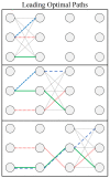
A layer by layer example of a classical approach to finding $W_{\min }$ or $W_{\max }$, for the case of $N=3$ and $L=4$. The blue-dashed, green-solid, and red-dotted lines each represent possible solutions for the optimal path ending on each of the three nodes per layer.

Figure 6

(top) An example geometry of size $N=2$, $L=4$. For the case of $N=2$, a single qubit is sufficient for representing all possible node choices per layer via the states $|0\rangle$ and $|1\rangle$. (bottom) An example geometry of size $N=4$, $L=4$, requiring two qubits for representing the nodes in each layer.

Figure 7

An example path (red-dashed) for a graph of size $N=2$, $L=4$. The quantum state $|0100\rangle$ represents the path shown in red, using the single qubit states $|0\rangle$ and $|1\rangle$ for bottom and top row nodes respectively.

Figure 8

(top) Illustration of layers i and j for an $N=2$ graph, and the four weighted edges shared between them. (bottom) Quantum circuit for achieving the $U_{ij}$ operation outlined in Equation (15).

Figure 9

The complete circuit design for $U_{\mathrm{P}}$, for the case of $N=2$. Each $U_{ij}$ operation applies the four ${\varphi }_i$ phases corresponding to the ${\omega }_i$ weights connecting layers i and j. Because of the way in which phases add exponentially, the order in which a total weight $W_i$ is applied to a state $|{\mathrm{P}}_i\rangle$ can be done in two sets of parallel operations, shown by the dashed-grey line.

Figure 10

(top) A sequential bipartite graph of varying N at each layer. (bottom) A mixed qudit quantum state capable of representing all possible paths through the geometry.

Figure 11

Quantum circuits for $U_{ij}$ connecting two layers of $N=4$ nodes. (top) A qubit-based quantum circuit (bottom) A $d=4$ qudit-based quantum circuit. More information on qudit unitary operations and circuits can be found in the review study by Wang et al. [54], such as the $X_d^{-}$ operator shown here.

Figure 12

Histograms of $W_i$ for randomly generated graphs of various N and L sizes, with $R=100$. As N and L increase while keeping R constant, the profile of these $\mathbb{W}$ distributions approach perfect gaussians, given by Equation (18).

Figure 13

(black circles/blue lines) A histogram of $\mathbb{W}$ for a randomly generated graph with parameters: $N=6$, $L=10$, $R=100$. (red dash) A best-fit gaussian plot of the form given in Equation (18), minimizing Equation (19) (R_corr ≈ 3.981), with gaussian parameter values reported in the top-right.

Figure 14

(left) An example histogram of all $W_i$ paths for the case of $N=4$, $L=10$, $R=100$. (right) The same distribution mapped to a complete $2\pi$ cycle of phases via the cost oracle $U_{\mathrm{P}}$ acting on the equal superposition state $|\mathrm{s}\rangle$. Additionally, the resulting mean (red ‘X’) and $|{\mathrm{P}}_{\min }\rangle$/$|{\mathrm{P}}_{\max }\rangle$ states (blue diamond) are shown. An accompanying color scale is provided on the far right, illustrating the percentile distribution of states for both plots.

Figure 15

Examples of amplitude amplification, comparing the use of $U_{\mathrm{P}}$ vs. $U_{\mathrm{G}}$ for five iterations, both with the same number of total states $N^{\prime }$ = 24,000. In both plots, the origin (0,0) (black ‘+’), the mean point (red ‘x’), the desired boosted state (blue diamond), and all other points (black circles) are shown. For scale, the radius of the equal superposition state $|\mathrm{s}\rangle$ (blue circle) is also shown ($1/\sqrt{N^{\prime }}$), as well as the probability of measuring the blue diamond state (which can be used to infer distance to the origin).

Figure 16

A comparison of probability boosting using $U_{\mathrm{G}}$ (blue-dashed) vs. $U_{\mathrm{P}}$ (red-solid) as a function of steps (oracle + diffusion iterations), both acting on a quantum system of $6^{10}$ states. For $U_{\mathrm{G}}$ we track the probability of the marked state, while the $U_{\mathrm{P}}$ case tracks the probability of measuring $|{\mathrm{P}}_{\min }\rangle$.

Figure 17

(1–3) Illustrations of how our python-based simulator creates gaussian $\mathbb{W}$ distributions for testing. In step 1, we pick a standard deviation $\sigma$ and create a continuous gaussian from 0 to $2\pi$, with $\alpha =1$ and $\mu =\pi$. In step 2 we select how many unique $W_i$ phases we want to model, and use this number to discretize the continuous gaussian into two discrete arrays $G_{\mathrm{x}}$ and $G_{\mathrm{y}}$. In step 3 we select a target Hilbert space size N to model, and scale all of the values in $G_{\mathrm{y}}$ up to integers, such that the sum($G_{\mathrm{y}}$) is as close to N as possible. And finally in step 4 we similuate amplitude amplification using $G_{\mathrm{x}}$ and $G_{\mathrm{y}}$, tracking the probability of $|{\mathrm{P}}_{\min }\rangle$.

Figure 18

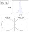
(top) An example distribution created from our simulator, before rounding in stage 3, with properties of the distribution given on the left. (bottom) Two different $U_{\mathrm{P}}$ interpretations of the distribution shown on top. (left) The long tail model, whereby all values of $G_{\mathrm{y}}$ are rounded up to the nearest integer. Grey dashes indicate the region where pop($W_i$) $=1$. (right) The short tail model where all values are rounded down, causing pop($W_i$) values near the tails to be zero for small $\sigma$.

Figure 19

Results for simulated gaussian distributions of Hilbert space size $N=60·{10}^6$, following the long tail model, as a function of standard deviation $\sigma$. (top) Black data points indicate the highest achievable probabilities $P_{\mathrm{M}}$ for $|{\mathrm{P}}_{\min }\rangle$, while the red-dashed line shows $P_{\mathrm{M}}·$pop($W_{\min }$) for cases with multiple $W_{\min }$ solutions. (bottom) The number of required iterations $S_{\mathrm{M}}$ in order to reach $P_{\mathrm{M}}$.

Figure 20

(top left) An example distribution created from our simulator following the short tail model, causing $W_{\min }$ and $W_{\max }$ to be located away from 0 and $2\pi$. (top right) The same distribution scaled by $p_{\mathrm{s}}$ to a full $2\pi$ range. (bottom) Below each histogram distribution is an amplitude space plot of $U_{\mathrm{P}}|s\rangle$, tracking the location of $|{\mathrm{P}}_{\min }\rangle$ (blue diamond) and the mean point (red ‘X’).

Figure 21

Results for simulated gaussian distributions of various Hilbert space sizes (blue = $60·{10}^6$, orange = $10·{10}^6$, and green = $2·{10}^6$), following the short tail model, as a function of initial standard deviation $\sigma$. (left) $P_{\mathrm{M}}$ and $S_{\mathrm{M}}$ plots for boosting $|{\mathrm{P}}_{\min }\rangle$. (top right) The standard deviation ${\sigma }^{\prime }$ after rescaling each distribution by the $p_{\mathrm{s}}$ value which maximizes $P_{\mathrm{M}}$ (see Figure 20). (bottom right) The total number of unique $W_i$ phases modeled by each distribution.

Figure 22

A plot of $p_{\mathrm{s}}$ vs. achievable probabilities via amplitude amplification, for the $\mathbb{W}$ distribution shown in Figure 13. The state $|{\mathrm{P}}_{\min }\rangle$ represents the solution to the pathfinding problem $W_{\min }$, while $|{\mathrm{P}}_{\min }^{\prime }\rangle$ corresponds to the next smallest $W_i$.

Figure 23

(top) An example $\mathbb{W}$ histogram distribution for the case $N=30$, $L=4$, $R=200$. (bottom) A plot of all $p_{\mathrm{s}}$ values used at each step in order to optimized the probability of measuring $|{\mathrm{P}}_{\min }\rangle$. Note the small black arrow, marking the $p_{\mathrm{s}}$ value at step 1. To the right of each plot are accompanying details about the success of each amplitude amplification process for each approach.

Figure 24

Results from testing on 100 randomly generated $\mathbb{W}$ distributions, for $N=6$, $L=10$, $R=100$. For each trial, we report the highest $P_{\mathrm{M}}$ probability found for the state $|{\mathrm{P}}_{\min }\rangle$ using (light blue) a step-varying $p_{\mathrm{s}}$ approach, (green) a single optimal $p_{\mathrm{s}}$ approach, and (dark red) an average $p_{\mathrm{s}}$ approach. Reported on the right side of the figure are the averages found for all three approaches.

Figure 25

(left) Geometric structure for the Traveling Salesman Problem, for the case $N=8$. Each edge contains a weighted value $w_{jk}$, where j and k are the two connected nodes. (right) An example path, touching each node exactly once. Each path ${\mathrm{P}}_i$ is defined by a unique ordering of all N nodes ($N!$ in total), with $W_i$ corresponding to the sum of all weighted edges composing the path.

Figure 26

(left) Geometric illustrations for 12 of the possible solution paths for an $N=4$ TSP weighted graph. (right) Quantum state representations for the 12 paths shown, plus 12 additional states with opposite direction.

Figure 27

Spanning tree representation of all possible paths for an $N=4$ Traveling Salesman problem.

Figure 28

(leftmost) Initial mapping of an $N=5$ TSP to the quantum states $|0\rangle$–$|4\rangle$, and their accompanying city names. (panels 1–4) Step by step outline of two different paths through the geometry, illustrating the ‘clockwise’ nomenclature outlined in this section. At each step, the path thus far is illustrated in solid black lines/states, while potential next nodes are shown in blue arrows/states.

Figure 29

Results from using a single optimal $p_{\mathrm{s}}$ for randomly generated TSP weighted graphs as a function of problem size N, $R=100$. (dots) Average values for ${\sigma }^{\prime }$ (black) and $P_{\mathrm{M}}$ (blue). (bars) Intervals indicating the top $90\%$ of all $P_{\mathrm{M}}$ values found.

References

1. Grover L.K. A fast quantum mechanical algorithm for database search. arXiv. 19969605043
1. Boyer M., Brassard G., Hoyer P., Tapp A. Tight bounds on quantum searching. Fortschr. Phys. 1998;46:493–506. doi: 10.1002/(SICI)1521-3978(199806)46:4/5<493::AID-PROP493>3.0.CO;2-P. - DOI
1. Bennett C.H., Bernstein E., Brassard G., Vazirani U. Strengths and Weaknesses of Quantum Computing. Siam J. Comput. 1997;26:1510–1523. doi: 10.1137/S0097539796300933. - DOI
1. Farhi E., Gutmann S. Analog analogue of a digital quantum computation. Phys. Rev. A. 1998;57:2403. doi: 10.1103/PhysRevA.57.2403. - DOI
1. Brassard G., Hoyer P., Tapp A. Quantum Counting; Proceedings of the LNCS 1443: 25th International Colloquium on Automata, Languages, and Programming (ICALP); Aalborg, Denmark. 13–17 July 1998; pp. 820–831.
LinkOut - more resources