Sorting of Odor Dilutions Is a Meaningful Addition to Assessments of Olfactory Function as Suggested by Machine-Learning-Based Analyses

Abstract

Background: The categorization of individuals as normosmic, hyposmic, or anosmic from test results of odor threshold, discrimination, and identification may provide a limited view of the sense of smell. The purpose of this study was to expand the clinical diagnostic repertoire by including additional tests.

Methods: A random cohort of n = 135 individuals (83 women and 52 men, aged 21 to 94 years) was tested for odor threshold, discrimination, and identification, plus a distance test, in which the odor of peanut butter is perceived, a sorting task of odor dilutions for phenylethyl alcohol and eugenol, a discrimination test for odorant enantiomers, a lateralization test with eucalyptol, a threshold assessment after 10 min of exposure to phenylethyl alcohol, and a questionnaire on the importance of olfaction. Unsupervised methods were used to detect structure in the olfaction-related data, followed by supervised feature selection methods from statistics and machine learning to identify relevant variables.

Results: The structure in the olfaction-related data divided the cohort into two distinct clusters with n = 80 and 55 subjects. Odor threshold, discrimination, and identification did not play a relevant role for cluster assignment, which, on the other hand, depended on performance in the two odor dilution sorting tasks, from which cluster assignment was possible with a median 100-fold cross-validated balanced accuracy of 77-88%.

Conclusions: The addition of an odor sorting task with the two proposed odor dilutions to the odor test battery expands the phenotype of olfaction and fits seamlessly into the sensory focus of standard test batteries.

Keywords: data science; machine learning; olfaction; olfactory testing; patients.

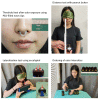
Figure 1

Photographs showing details of the administration of olfactory tasks. Top left–nasal clip (see also insert) filled with phenylethylalcohol to provide continuous olfactory background stimulation. Top right—distance test with an opened jar with peanut butter slowly moved upwards towards the nose of the blinded participant with a meter to measure the distance from the nares. Bottom left—lateralization task using a hand-held squeezing device (see also inserts), which allows to administer the same amount of air to the left and right nostrils of the blinded participant with one bottle containing eucalyptus. Bottom right—odor-sorting task with the participant arranging odor-containing bottles according to the different odor intensities with odor concentrations indicated at the bottom of the bottle (see also insert).

Figure 2

Raw non-transformed and non-imputed olfaction-related data acquired from n = 135 individuals. Single data points are plotted as dots on violin plots showing the probability density distribution of the variables, and in addition, boxplots provide basic descriptive statistics. Variable names, if not self-explaining: “olfthresh“ = olfactory threshold to phenyl ethyl alcohol (PEA), “olfdis” = score in the odor discrimination task, “olfident” = score in the odor identification task. Higher values indicate better olfactory performance. “log Distance right/left nostril” = perception of peanut butter odor from a distance, “Score PEA/EUG” = scores in the odor sorting tasks, “Lat correct assignments overall” score in the lateralization test. Lower values indicate better olfactory performance. The figure has been created using Python version 3.8.12 for Linux (https://www.python.org, accessed on 28 January 2022) and Seaborn Python data visualization library (https://seaborn.pydata.org, accessed on 28 January 2022 [65]).

Figure 3

Correlations of olfaction-related data collected from n = 135 subjects, transformed to normal distribution and with missing values imputed. Age and BMI were additionally included. The correlation matrix is color-coded according to the strength and direction of the correlation. Each cell is labeled with the value of Pearson’s r in black numbers. If the correlation is significant, the p-value is indicated in red numbers below the correlation coefficient. The diagonal of the correlations of each variable with itself has been omitted. Variables belonging to the same subtest are highlighted by black rectangles to increase distinction of intra- and intertest correlations. Olfactory variables are outlined in red. Variable names, if not self-explaining: “olfthresh“ = olfactory threshold to phenyl ethyl alcohol (PEA), “olfdis” = score in the odor discrimination task, “olfident” = score in the odor identification task, “log Distance right/left nostril” = perception of peanut butter odor from a distance, “Score PEA/EUG” = scores in the odor sorting tasks, “Lat correct assignments overall” score in the lateralization test. The figure has been created using Python version 3.8.12 for Linux (https://www.python.org, accessed on 28 January 2022) and Seaborn Python data visualization library (https://seaborn.pydata.org, accessed on 28 January 2022 [65]).

Figure 4

Results of a principal component analysis (PCA)-based projection of centered and standardized olfaction-related data. (a) Projection of olfactory data collected in d = 15 olfactory variables from n = 135 subjects onto the first two principal component levels. Data points originating from subjects with normosmia or hyposmia are colored red and blue, respectively. (b) Line plot of cumulative explained variance with increasing number of principal components (PCs). (c) Bar graph of the eigenvalues of each of the 15 PCs. Seven PCs had an eigenvalue > 1 and were selected for further data analysis such as clustering. The overlaid biplot (red lines) shows the variables as vectors in the PC projection space. (d) Contribution of each variable to the principal components, normalized for the contribution of each PC to the explanation of the total variance. The lighter blue bars show the significance of the variables across the entire PC space, while the darker blue bars overlaying them show the contribution when only the relevant 7 PCs are considered. The 6 dark blue bars indicate those selected by item categorization using computed ABC analysis as the most informative variables placed in ABC set “A”. The bar chart shows the column sums of the heat map shown below in panel (e) Z-normalized correlation matrix between the original z-transformed dataset and the PC space, normalized by the explained variance. The figure has been created using Python version 3.8.12 for Linux (https://www.python.org, accessed on 28 January 2022) and Seaborn Python data visualization library (https://seaborn.pydata.org, accessed on 28 January 2022 [65]).

Figure 5

Clustering of the d = 15 olfaction-related parameters. (a) Factorial plot of the individual data points on a principal components map, obtained following k-means clustering. The colored areas visualize the cluster separation. The cluster members are connected by straight lines with their respective cluster centers. (b) Silhouette plot associated with the cluster solution presented in panel (a). The horizontal bars show the average distance of each data point in a cluster is to points in neighboring cluster(s), scaled in the range of [−1, 1] [48]. The figure has been created using Python version 3.8.12 for Linux (https://www.python.org, accessed on 28 January 2022) and Seaborn Python data visualization library (https://seaborn.pydata.org, accessed on 28 January 2022 [65]).

Figure 6

Differences of the d = 15 olfaction-related variables between the two k-means clusters. (a) Effect size calculated as Cohen’s d for the parameters used for clustering, and age and the reciprocal square transformed BMI as demographic parameters of known or possible interest of an olfactory context. The effect size of Cohen’s d > 0.2, > 0.5 or > 0.8 generally regarded as small, medium, or large effects are indicated as horizontal dotted lines. Positive values indicate larger values in cluster 1 than in cluster 0. The variables with the most relevant effect sizes according to item categorization (see panel d) are plotted in darker blue color. Variable names, if not self-explaining: “olfthresh“ = olfactory threshold to phenyl ethyl alcohol (PEA), “olfdis” = score in the odor discrimination task, “olfident” = score in the odor identification task. Higher values indicate better olfactory performance. “log Distance right/left nostril” = perception of peanut butter odor from a distance, “Score PEA/EUG” = scores in the odor sorting tasks, “Lat correct assignments overall” score in the lateralization test. Lower values indicate better olfactory performance. (b) Z Individual data points, z-transformed to enhance visualization of group differences across different original scales of the values, plotted as dots on violin plots showing the probability density distribution of the variables, and in addition, boxplots provide basic descriptive statistics. Statistical significance of the differences between the clusters for each variable was analyzed by performing Mann–Whitney U-tests. The obtained p-values are shown above the respective variables, with color coding for black = “not significant”, p > 0.05), blue = “significant but not passing α correction”, red = “significant with α correction”. (c) Mosaic plot of the contingency table of cluster membership (x-axis) versus olfactory diagnosis of hyposmia or normosmia (y-axis). (d) ABC analysis plot (blue line) showing the cumulative distribution function of the absolute effect sizes, along with the identity distribution, x_i = constant (magenta line), i.e., each variable has the same effect in terms of inter-cluster differences, and the uniform distribution, i.e., each variable had the same chance to distinguish between cluster (for further details about computed ABC analysis, see [44]). The red lines indicate the borders between ABC subsets “A”, “B”, and “C”. Subset “A” containing d = 6 variables is regarded as containing the most relevant variables for cluster distinction (marked in darker blue in panel a). The figure has been created using Python version 3.8.12 for Linux (https://www.python.org, accessed on 28 January 2022) and Seaborn Python data visualization library (https://seaborn.pydata.org, accessed on 28 January 2022 [65]) and our Python package “ABCanalysis” (https://github.com/JornLotsch/ABCanalysis, accessed on 28 January 2022).

Figure 7

Identification of the variables that were most informative in assigning a subject to the k-means clusters. Feature selection by 17 different methods listed in Table 1. (a) The sum score of selections of each variable across the methods was subjected to a computed ABC analysis to identify the most informative variables for all methods of feature selection (row sums in Table 1). The darker blue bars indicate the variables selected for the reduced feature set resulting from ABC analysis-based item categorization. (b) ABC analysis plot (blue line) showing the cumulative distribution function of the sums of occurrences in ABC category “A” in the ABC analyses previously performed with each feature selection method separately. The red lines show the boundaries between the ABC subsets “A”, “B” and “C”. Category “A” with d = 6 variables is considered to include the most relevant variables for cluster discrimination (marked in darker blue in panel a). The figure was created using Python version 3.8.12 for Linux (https://www.python.org, accessed on 28 January 2022), with the seaborn statistical data visualization package (https://seaborn.pydata.org, accessed on 28 January 2022 [65]) and our Python package “ABCanalysis” (https://github.com/JornLotsch/ABCanalysis, accessed on 28 January 2022). Variable names, if not self-explaining: “olfthresh“ = olfactory threshold to phenyl ethyl alcohol (PEA), “olfdis” = score in the odor discrimination task, “olfident” = score in the odor identification task, log Distance right/left nostril” = perception of peanut butter odor from a distance, “Score PEA/EUG” = scores in the odor sorting tasks, “Lat correct assignments overall” score in the lateralization test.

Figure 8

Differences in sum scores of selections of each variable across 17 feature selection methods when the target was the olfaction-related cluster versus the target defined as the olfactory diagnosis of normosmia or hyposmia. The variables selected as informative for the cluster structure are plotted in darker blue. The figure has been created using Python version 3.8.12 for Linux (https://www.python.org, accessed on 28 January 2022) and Seaborn Python data visualization library (https://seaborn.pydata.org, accessed on 28 January 2022 [65]) and our Python package “ABCanalysis” (https://github.com/JornLotsch/ABCanalysis, accessed on 28 January 2022). Variable names, if not self-explaining: “olfthresh“ = olfactory threshold to phenyl ethyl alcohol (PEA), “olfdis” = score in the odor discrimination task, “olfident” = score in the odor identification task, log Distance right/left nostril” = perception of peanut butter odor from a distance, “Score PEA/EUG” = scores in the odor sorting tasks, “Lat correct assignments overall” score in the lateralization test.

References

1. Kobal G., Hummel T., Sekinger B., Barz S., Roscher S., Wolf S.R. “Sniffin’ Sticks”: Screening of olfactory performance. Rhinology. 1996;34:222–226. - PubMed
1. Hummel T., Sekinger B., Wolf S.R., Pauli E., Kobal G. ‘Sniffin’ sticks’: Olfactory performance assessed by the combined testing of odor identification, odor discrimination and olfactory threshold. Chem. Senses. 1997;22:39–52. doi: 10.1093/chemse/22.1.39. - DOI - PubMed
1. Cain W.S., Gent J.F., Goodspeed R.B., Leonard G. Evaluation of olfactory dysfunction in the Connecticut Chemosensory Clinical Research Center (CCCRC) Laryngoscope. 1988;98:83–88. doi: 10.1288/00005537-198801000-00017. - DOI - PubMed
1. Thomas-Danguin T., Rouby C., Sicard G., Vigouroux M., Farget V., Johanson A., Bengtzon A., Hall G., Ormel W., De Graaf C., et al. Development of the ETOC: A European test of olfactory capabilities. Rhinology. 2003;41:142–151. - PubMed
1. Lam H.C., Sung J.K., Abdullah V.J., van Hasselt C.A. The combined olfactory test in a Chinese population. J. Laryngol. Otol. 2006;120:113–116. doi: 10.1017/S0022215105003889. - DOI - PubMed
LinkOut - more resources