Machine Learning and Pharmacometrics for Prediction of Pharmacokinetic Data: Differences, Similarities and Challenges Illustrated with Rifampicin

Abstract

Pharmacometrics (PM) and machine learning (ML) are both valuable for drug development to characterize pharmacokinetics (PK) and pharmacodynamics (PD). Pharmacokinetic/pharmacodynamic (PKPD) analysis using PM provides mechanistic insight into biological processes but is time- and labor-intensive. In contrast, ML models are much quicker trained, but offer less mechanistic insights. The opportunity of using ML predictions of drug PK as input for a PKPD model could strongly accelerate analysis efforts. Here exemplified by rifampicin, a widely used antibiotic, we explore the ability of different ML algorithms to predict drug PK. Based on simulated data, we trained linear regressions (LASSO), Gradient Boosting Machines, XGBoost and Random Forest to predict the plasma concentration-time series and rifampicin area under the concentration-versus-time curve from 0-24 h (AUC_0-24h) after repeated dosing. XGBoost performed best for prediction of the entire PK series (R²: 0.84, root mean square error (RMSE): 6.9 mg/L, mean absolute error (MAE): 4.0 mg/L) for the scenario with the largest data size. For AUC_0-24h prediction, LASSO showed the highest performance (R²: 0.97, RMSE: 29.1 h·mg/L, MAE: 18.8 h·mg/L). Increasing the number of plasma concentrations per patient (0, 2 or 6 concentrations per occasion) improved model performance. For example, for AUC_0-24h prediction using LASSO, the R² was 0.41, 0.69 and 0.97 when using predictors only (no plasma concentrations), 2 or 6 plasma concentrations per occasion as input, respectively. Run times for the ML models ranged from 1.0 s to 8 min, while the run time for the PM model was more than 3 h. Furthermore, building a PM model is more time- and labor-intensive compared with ML. ML predictions of drug PK could thus be used as input into a PKPD model, enabling time-efficient analysis.

Keywords: feature selection; machine learning; pharmacokinetics; pharmacometrics; population pharmacokinetics; rifampicin; simulation.

Figure 1

Overall proposed workflow. Blue panels indicate pharmacometrics and yellow machine learning.

Figure 2

Illustration of a two-compartment pharmacokinetic model for a fictive drug. A_GI, amount of drug in the gastrointestinal tract; k₀₁, absorption rate constant; k₁₀, elimination rate constant; k₁₂, rate constant describing distribution from central to peripheral compartment; k₂₁, rate constant describing distribution from peripheral to central compartment; V₁, volume of central compartment (e.g., blood); V₂, volume of peripheral compartment (e.g., brain tissue). Drug clearance is expressed as $k_{10}\times {\mathrm{V}}_1$.

Figure 3

Comparison of the general model development workflow between pharmacometrics and machine learning. The different colors represent different steps of model development. Green: data preparation, blue: model building, red: model evaluation, orange: finalizing the model.

Figure 4

Importance scores for evaluated features shown for the different machine learning algorithms. (A) GBM, (B) Random Forest and (C) XGBoost using features only (scenario 1) as input for prediction of plasma concentration versus time. The error bars represent the standard deviation. AGE, age (years); BMI, body mass index (kg/m²); DOSE, daily rifampicin dose (mg); FFM, fat-free mass (kg); HIV, HIV-coinfection; HT, body height (cm); OCC, treatment week; RACE, race; SEX, gender; TAD, time after dose (h); WT, bodyweight (kg).

Figure 4

Importance scores for evaluated features shown for the different machine learning algorithms. (A) GBM, (B) Random Forest and (C) XGBoost using features only (scenario 1) as input for prediction of plasma concentration versus time. The error bars represent the standard deviation. AGE, age (years); BMI, body mass index (kg/m²); DOSE, daily rifampicin dose (mg); FFM, fat-free mass (kg); HIV, HIV-coinfection; HT, body height (cm); OCC, treatment week; RACE, race; SEX, gender; TAD, time after dose (h); WT, bodyweight (kg).

Figure 5

Predictions of rifampicin plasma concentration-time series from the different ML algorithms compared to the simulations from the population PK model, considered to be observations in this study. Panel (A) is the scenario where the model was trained to predict the rifampicin plasma concentration-time series using features only as input. In panel (B), the models were trained to predict the rifampicin plasma concentration-time series based on features and 2 plasma concentrations at time-points 2 and 4 h post-dose at days 7 and 14. In panel (C), the models were trained to predict the rifampicin plasma concentration-time series based on features and 6 plasma concentrations at time-points 0.5, 1, 2, 4, 8 and 24 h post-dose at days 7 and 14. The red dashed line represents a trendline through the data. The black solid line is the line of identity, indicating 100% agreement between true and predicted values.

Figure 5

Predictions of rifampicin plasma concentration-time series from the different ML algorithms compared to the simulations from the population PK model, considered to be observations in this study. Panel (A) is the scenario where the model was trained to predict the rifampicin plasma concentration-time series using features only as input. In panel (B), the models were trained to predict the rifampicin plasma concentration-time series based on features and 2 plasma concentrations at time-points 2 and 4 h post-dose at days 7 and 14. In panel (C), the models were trained to predict the rifampicin plasma concentration-time series based on features and 6 plasma concentrations at time-points 0.5, 1, 2, 4, 8 and 24 h post-dose at days 7 and 14. The red dashed line represents a trendline through the data. The black solid line is the line of identity, indicating 100% agreement between true and predicted values.

Figure 5

Predictions of rifampicin plasma concentration-time series from the different ML algorithms compared to the simulations from the population PK model, considered to be observations in this study. Panel (A) is the scenario where the model was trained to predict the rifampicin plasma concentration-time series using features only as input. In panel (B), the models were trained to predict the rifampicin plasma concentration-time series based on features and 2 plasma concentrations at time-points 2 and 4 h post-dose at days 7 and 14. In panel (C), the models were trained to predict the rifampicin plasma concentration-time series based on features and 6 plasma concentrations at time-points 0.5, 1, 2, 4, 8 and 24 h post-dose at days 7 and 14. The red dashed line represents a trendline through the data. The black solid line is the line of identity, indicating 100% agreement between true and predicted values.

Figure 6

Prediction interval visual predictive check for the best-performing model (XGBoost) trained using 6 plasma concentrations as input (scenario 3) shown for the whole population. Open circles are the rifampicin plasma concentrations simulated from the population PK model, considered to be observed data in this study. The shaded area is the 95th prediction interval of the machine learning model predictions (XGBoost) and the solid blue line is the median of the model predictions. The upper and lower red dashed lines are the 97.5th and 2.5th percentiles of the observed data, respectively, and the solid red line is the median of the observed data.

Figure 7

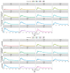
Individual rifampicin plasma concentrations predicted from the XGBoost model (solid line and open circles) compared to the concentrations simulated from the population PK model, considered to be observations in this study (black closed circles) shown for scenario 3 (features and 6 plasma concentrations used for prediction) for 15 randomly selected IDs. Panel (A) represents the predictions for each individual in the test dataset at day 7. Panel (B) represents the predictions for each individual in the test dataset at day 14. The different colors indicate the different daily rifampicin doses.

Figure 8

Visual predictive check for the re-estimated population PK model based on the simulated data. Open blue circles are the rifampicin plasma concentrations simulated from the population PK model, considered to be observed data in this study. The upper and lower dashed lines are the 95th and 5th percentiles of the observed data, respectively, and the solid line is the median of the observed data. The shaded areas (top to bottom) are the 95% confidence intervals of the 95th (blue shaded area), median (red shaded area) and 5th (blue shaded area) percentiles of the simulated data.

Figure 9

Predictions of rifampicin AUC_0–24h at days 7 and 14 from the different ML algorithms compared to the NCA derived AUC_0–24h, considered to be observations in this study. Panel (A) is the scenario where the model was trained using features only as input. In panel (B), the models were trained to predict rifampicin AUC_0–24h based on features and 2 plasma concentrations at time-points 2 h and 4 h post-dose at days 7 and 14. In panel (C), the models were trained to predict rifampicin AUC_0–24h based on features and 6 plasma concentrations at time-points 0.5 h, 1 h, 2 h, 4 h, 8 h and 24 h post-dose at days 7 and 14. The red dashed line represents a trendline through the data. The black solid line is the line of identity, indicating 100% agreement between true and predicted values.

Figure 9

Predictions of rifampicin AUC_0–24h at days 7 and 14 from the different ML algorithms compared to the NCA derived AUC_0–24h, considered to be observations in this study. Panel (A) is the scenario where the model was trained using features only as input. In panel (B), the models were trained to predict rifampicin AUC_0–24h based on features and 2 plasma concentrations at time-points 2 h and 4 h post-dose at days 7 and 14. In panel (C), the models were trained to predict rifampicin AUC_0–24h based on features and 6 plasma concentrations at time-points 0.5 h, 1 h, 2 h, 4 h, 8 h and 24 h post-dose at days 7 and 14. The red dashed line represents a trendline through the data. The black solid line is the line of identity, indicating 100% agreement between true and predicted values.

Figure 9

Predictions of rifampicin AUC_0–24h at days 7 and 14 from the different ML algorithms compared to the NCA derived AUC_0–24h, considered to be observations in this study. Panel (A) is the scenario where the model was trained using features only as input. In panel (B), the models were trained to predict rifampicin AUC_0–24h based on features and 2 plasma concentrations at time-points 2 h and 4 h post-dose at days 7 and 14. In panel (C), the models were trained to predict rifampicin AUC_0–24h based on features and 6 plasma concentrations at time-points 0.5 h, 1 h, 2 h, 4 h, 8 h and 24 h post-dose at days 7 and 14. The red dashed line represents a trendline through the data. The black solid line is the line of identity, indicating 100% agreement between true and predicted values.

References

1. Upton R.N., Mould D.R. Basic Concepts in Population Modeling, Simulation, and Model-Based Drug Development: Part 3—Introduction to Pharmacodynamic Modeling Methods. CPT Pharmacomet. Syst. Pharmacol. 2014;3:e88. doi: 10.1038/psp.2013.71. - DOI - PMC - PubMed
1. Meibohm B., Derendorf H. Basic concepts of pharmacokinetic/pharmacodynamic (PK/PD) modelling. Int. J. Clin. Pharmacol. Ther. 1997;35:401–413. - PubMed
1. Réda C., Kaufmann E., Delahaye-Duriez A. Machine learning applications in drug development. Comput. Struct. Biotechnol. J. 2020;18:241–252. doi: 10.1016/j.csbj.2019.12.006. - DOI - PMC - PubMed
1. McComb M., Bies R., Ramanathan M. Machine learning in pharmacometrics: Opportunities and challenges. Br. J. Clin. Pharmacol. 2021;88:1482–1499. doi: 10.1111/bcp.14801. - DOI - PubMed
1. Poynton M.R., Choi B., Kim Y., Park I., Noh G., Hong S., Boo Y., Kang S. Machine Learning Methods Applied to Pharmacokinetic Modelling of Remifentanil in Healthy Volunteers: A Multi-Method Comparison. J. Int. Med. Res. 2009;37:1680–1691. doi: 10.1177/147323000903700603. - DOI - PubMed
LinkOut - more resources