Model-based stationarity filtering of long-term memory data applied to resting-state blood-oxygen-level-dependent signal

Abstract

Resting-state blood-oxygen-level-dependent (BOLD) signal acquired through functional magnetic resonance imaging is a proxy of neural activity and a key mechanism for assessing neurological conditions. Therefore, practical tools to filter out artefacts that can compromise the assessment are required. On the one hand, a variety of tailored methods to preprocess the data to deal with identified sources of noise (e.g., head motion, heart beating, and breathing, just to mention a few) are in place. But, on the other hand, there might be unknown sources of unstructured noise present in the data. Therefore, to mitigate the effects of such unstructured noises, we propose a model-based filter that explores the statistical properties of the underlying signal (i.e., long-term memory). Specifically, we consider autoregressive fractional integrative process filters. Remarkably, we provide evidence that such processes can model the signals at different regions of interest to attain stationarity. Furthermore, we use a principled analysis where a ground-truth signal with statistical properties similar to the BOLD signal under the injection of noise is retrieved using the proposed filters. Next, we considered preprocessed (i.e., the identified sources of noise removed) resting-state BOLD data of 98 subjects from the Human Connectome Project. Our results demonstrate that the proposed filters decrease the power in the higher frequencies. However, unlike the low-pass filters, the proposed filters do not remove all high-frequency information, instead they preserve process-related higher frequency information. Additionally, we considered four different metrics (power spectrum, functional connectivity using the Pearson's correlation, coherence, and eigenbrains) to infer the impact of such filter. We provided evidence that whereas the first three keep most of the features of interest from a neuroscience perspective unchanged, the latter exhibits some variations that could be due to the sporadic activity filtered out.

Fig 1. Block diagram of the proposed method to filter resting-state BOLD data.

Fig 2. Mean value of the absolute AR(1) parameter averaged across all 98 subjects across all 4 runs.

Fig 3. Comparison between the generated noisy synthetic BOLD and the rs-BOLD signal from one of the ROI from dataset.

(A) The time series plot of the generated noisy synthetic BOLD (cyan-colored) and preprocessed rs-BOLD (dashed orange curve). (B) Power spectrum plot of the noisy synthetic BOLD (cyan) and rs-BOLD (orange).

Fig 4. Autocorrelation and normalised power spectrum plots of unfiltered and filtered synthetic BOLD signal.

(A) The designed synthetic BOLD signal with a sampling frequency of 1.3889 Hz (similar to the sampling rate of rs-fMRI HCP dataset) which has inverse power law autocorrelation plot (left panel) (similar to the observed original resting-state BOLD signal). The synthetic BOLD signal thus created consists of low frequency fluctuations in the range of 0.01 − 0.15 Hz (similar to the observation about intrinsic BOLD fluctuation in the resting brain in [9, 42, 43]), right panel. An artificial white noise is added to the created synthetic BOLD signal. (B) The left panel shows the sACF of the fractionally differenced (d = 2.6) synthetic BOLD signal (with white noise, WN(0, 100)). The right panel shows the normalised power spectrum plot of unfiltered dummy BOLD signal (cyan curve, WN(0, 100)) and the ARFIMA (1, 2.6, 0) filtered BOLD signal (dashed orange curved) embedded with zoomed in plot at higher frequency. (C) The sACF of the fractionally differenced (d = 3.8) synthetic BOLD signal (with white noise, WN(0, 10)) and normalised power spectrum plot of unfiltered dummy BOLD signal (cyan colored curve, WN(0, 10)) and the ARFIMA (1, 3.8, 0) filtered BOLD signal (dashed orange curve) embedded with zoomed in plot at higher frequency is depicted in the left and right panel respectively.

Fig 5. Normalised power spectrum of the unfiltered and filtered resting-state BOLD signal for three different ROIs.

The color-coded power spectrum plots, i.e. cyan and dashed orange, represent the plots of the resting-state BOLD signal and ARFIMA (1, d, 0) filtered BOLD signal respectively of one of the subjects. The location of each of the three ROI is presented in the brain overlay (in the centre) in different colours. The power spectrum of the corresponding ROI is outlined in the same colored box. (A-C) Normalised power spectrum of the resting-state and ARFIMA filtered BOLD signal corresponding to the ROI: 7 lying in the visual peripheral brain network (a green colored region in brain), ROI: 11 in the somatomotor auditory network of the brain (a blue colored region in the brain) and ROI: 37 in control network (a red colored region), respectively, is shown. The filter used in each of the case is: ARFIMA (1, 0.7, 0) (in A), ARFIMA (1, 0.3, 0) (in B) and ARFIMA (1, 0.5, 0) (in C).

Fig 6. Number of statistically distinguishable power spectrum (p < 0.05) in each ROI plotted on the brain overlays.

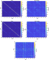
Fig 7. Whole brain FC matrix (comprising of 100 ROI) defined based on Pearson’s correlation.

The Pearson’s correlation FC matrix of each subject in each run is averaged across to find one representative FC matrix (mean ± std. deviation). (A) Pearson’s correlation matrix (mean ± std. deviation) (for 100 ROI) obtained from the resting-state BOLD time series. (B) Pearson’s correlation matrix (mean ± std. deviation) (for 100 ROI) obtained from the ARFIMA (1, d, 0) filtered BOLD time series. (C) The difference between the mean Pearson’s correlation matrix of the resting-state BOLD dataset(A) and the filtered BOLD time series of the whole brain (B).

Fig 8. Whole brain FC matrix (comprising of 100 ROI) based on the coherence.

The coherence FC matrix of each subject in each run is averaged across to find one representative FC matrix (mean ± std. deviation). (A) Coherence FC matrix (mean ± std. deviation) (for 100 ROI) obtained from the resting-state BOLD time series. (B) Coherence FC matrix (mean ± std. deviation) (for 100 ROI) obtained from the ARFIMA (1, d, 0) BOLD time series. (C) The difference between the mean coherence FC matrix of the resting-state BOLD dataset (A) and the filtered BOLD time series of the whole brain (B).

Fig 9. Clustering of eigenvectors and eigenvalues obtained from resting-state BOLD signal and ARFIMA (1, d, 0) (model-based) filtered resting-state BOLD signals.

All eigenvectors from all subjects were normalised and clustered into 5 clusters using k-means clustering. The clusters were color-coded across all subjects and all runs (98 subjects × 4 runs × 100 eigenmodes = 39,200 eigenvalues). The color codes blue, orange, yellow, purple and green correspond to cluster 1, 2, 3, 4 and 5, respectively. The plot in the centre shows the distribution of eigenvalues based on their frequency (the argument of eigenvalue) and stability (the absolute magnitude of eigenvalue) of resting-state and ARFIMA filtered BOLD signals. Error bars represent the mean and standard deviation of the average eigenvalue of each cluster. The eigenvalues are color coded based on the five identified clusters. The brain overlays in the left and right panel represent the spatial distribution of the eigenvector corresponding to the eigenvalue (same color coded) of resting-state BOLD signals before and after filtering, respectively. The cluster centroid (plotted on the brain overlays) were normalised by subtracting each centroid by its minimum element. Colorbar represents the normalised values of cluster centroid for each cluster (left and right panel).

Fig 10. Similarity between eigenvector centroid of the clusters and RSNs.

(A-B) denotes the spatial correlation between clusters and resting state networks before and after ARFIMA filtering on the resting-state BOLD data, respectively. The colorbar depicts the correlation values for both panels.

Fig 11. Comparison between the derived ARFIMA filter and first-order low-pass butterworth filter.

Both the figures show the comparison made on ROI: 11 corresponding to the somatomotor auditory region of the brain. (A) Normalised power spectrum of the unfiltered and filtered BOLD signal. The normalised power spectrum corresponding to the preprocessed resting-state BOLD signal is represented by the cyan curve, low-pass first-order butterworth filtered by yellow curve and the ARFIMA (1, 0.3, 0) filtered BOLD by the orange curve. (B) Magnitude bode plot of the transfer function of the low-pass first-order butterworth filter (yellow curve, cut off frequency: 0.1Hz) and the derived ARFIMA (1, 0.3, 0) filter (orange curve).

Fig 12. Amplification in the high frequencies for one of the ROI.

(A) shows the normalised power spectrum of the resting-state BOLD signal (cyan curve) and the ARFIMA filtered signal (dashed orange curve) for one of the ROI. (B) Magnitude bode plot of the derived ARFIMA filter (for the ROI shown in (A)) depicting amplification in higher frequencies.

References

1. Biswal B, Zerrin Yetkin F, Haughton VM, Hyde JS. Functional connectivity in the motor cortex of resting human brain using echo-planar MRI. Magnetic Resonance in Medicine. 1995;34(4):537–541. doi: 10.1002/mrm.1910340409 - DOI - PubMed
1. Lurie DJ, Kessler D, Bassett DS, Betzel RF, Breakspear M, Kheilholz S, et al.. Questions and controversies in the study of time-varying functional connectivity in resting fMRI. Network Neuroscience. 2020;4(1):30–69. doi: 10.1162/netn_a_00116 - DOI - PMC - PubMed
1. Monk CS, Peltier SJ, Wiggins JL, Weng SJ, Carrasco M, Risi S, et al.. Abnormalities of intrinsic functional connectivity in autism spectrum disorders. NeuroImage. 2009;47(2):764–772. doi: 10.1016/j.neuroimage.2009.04.069 - DOI - PMC - PubMed
1. Barkhof F, Haller S, Rombouts SA. Resting-state functional MR imaging: a new window to the brain. Radiology. 2014;272(1):29–49. doi: 10.1148/radiol.14132388 - DOI - PubMed
1. Guo W, Yao D, Jiang J, Su Q, Zhang Z, Zhang J, et al.. Abnormal default-mode network homogeneity in first-episode, drug-naive schizophrenia at rest. Progress in Neuro-Psychopharmacology and Biological Psychiatry. 2014;49:16–20. doi: 10.1016/j.pnpbp.2013.10.021 - DOI - PubMed
Publication types