Forest tree species distribution for Europe 2000-2020: mapping potential and realized distributions using spatiotemporal machine learning

Abstract

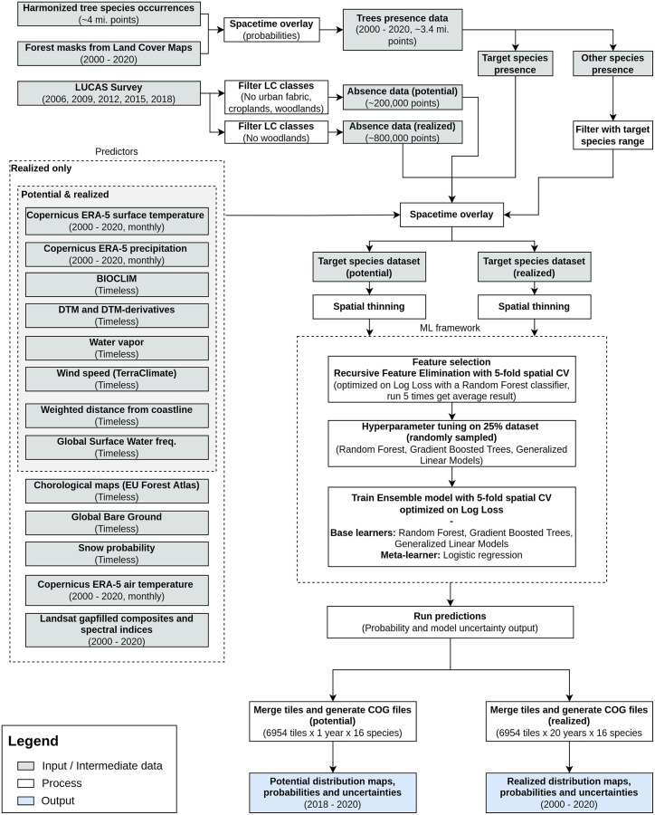
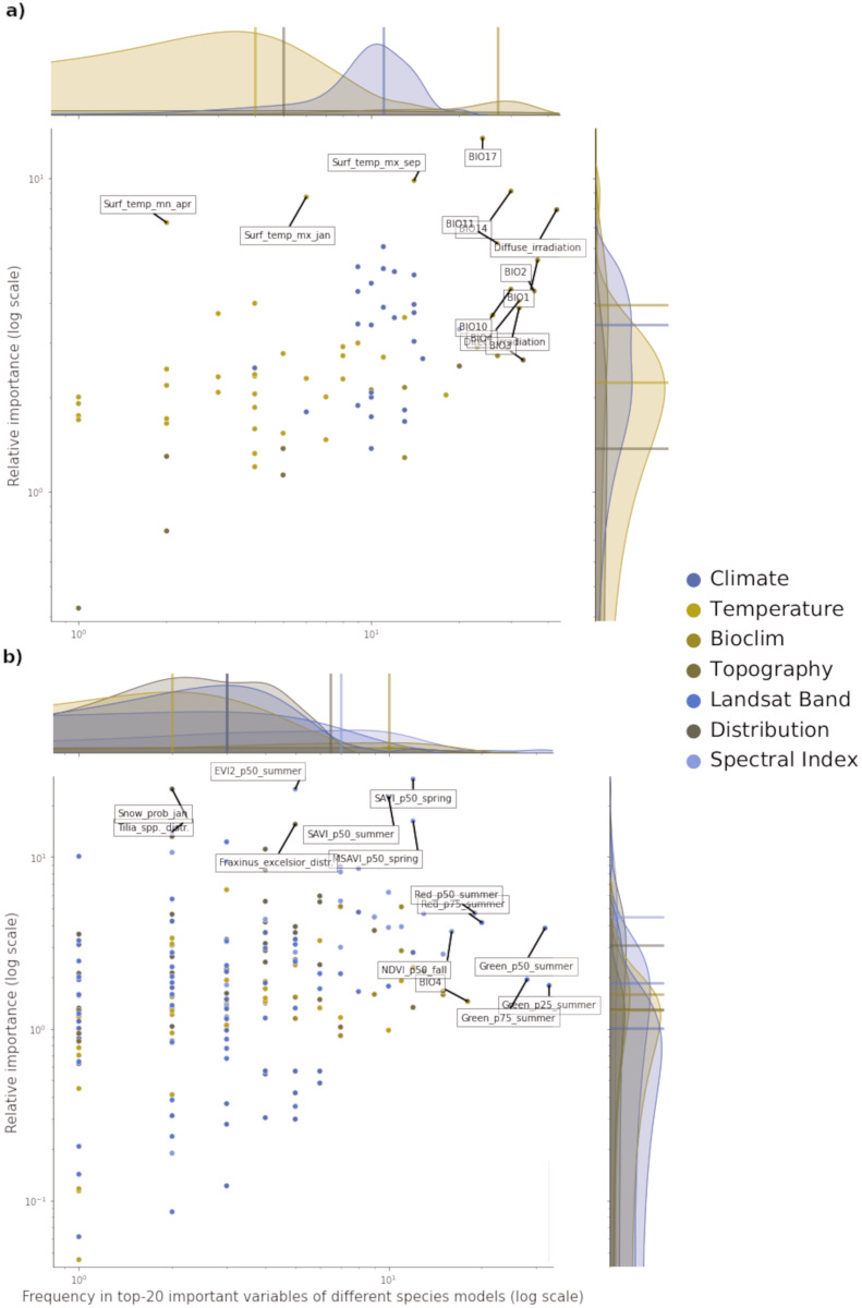
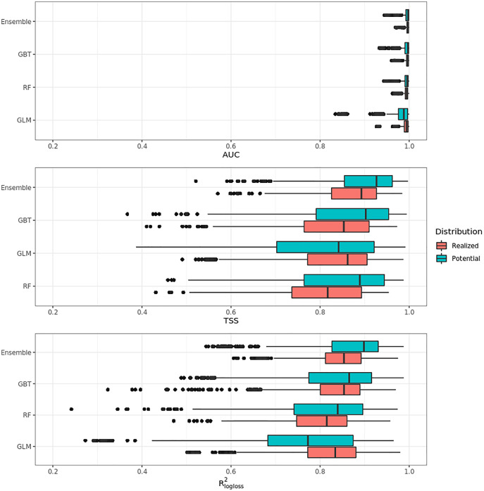
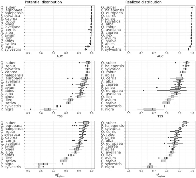
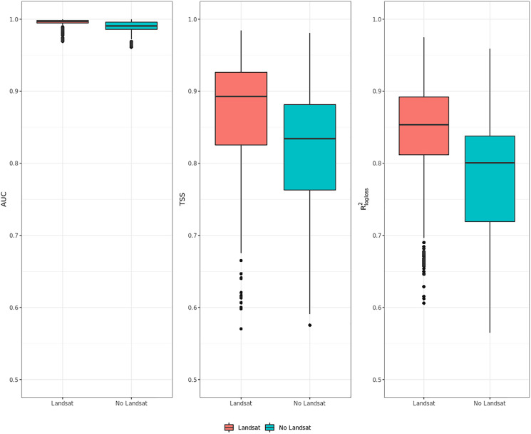
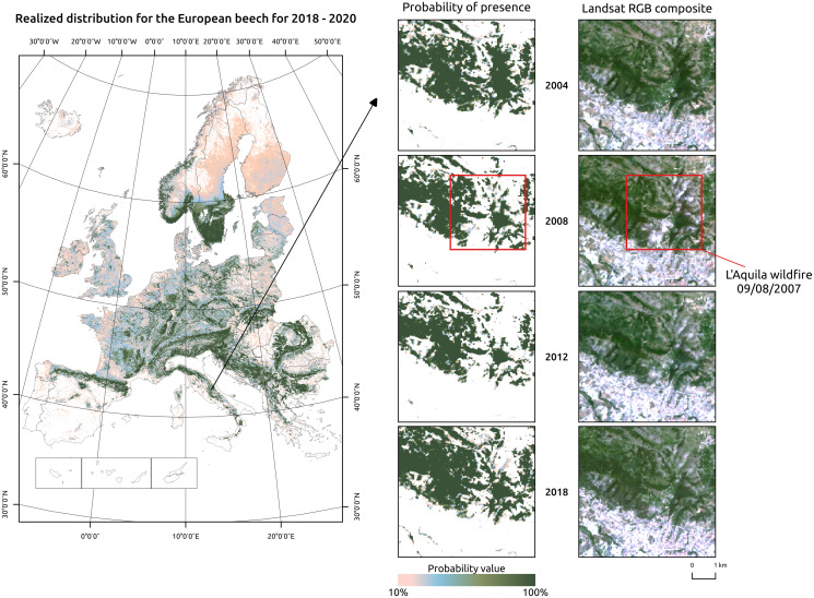
This article describes a data-driven framework based on spatiotemporal machine learning to produce distribution maps for 16 tree species (Abies alba Mill., Castanea sativa Mill., Corylus avellana L., Fagus sylvatica L., Olea europaea L., Picea abies L. H. Karst., Pinus halepensis Mill., Pinus nigra J. F. Arnold, Pinus pinea L., Pinus sylvestris L., Prunus avium L., Quercus cerris L., Quercus ilex L., Quercus robur L., Quercus suber L. and Salix caprea L.) at high spatial resolution (30 m). Tree occurrence data for a total of three million of points was used to train different algorithms: random forest, gradient-boosted trees, generalized linear models, k-nearest neighbors, CART and an artificial neural network. A stack of 305 coarse and high resolution covariates representing spectral reflectance, different biophysical conditions and biotic competition was used as predictors for realized distributions, while potential distribution was modelled with environmental predictors only. Logloss and computing time were used to select the three best algorithms to tune and train an ensemble model based on stacking with a logistic regressor as a meta-learner. An ensemble model was trained for each species: probability and model uncertainty maps of realized distribution were produced for each species using a time window of 4 years for a total of six distribution maps per species, while for potential distributions only one map per species was produced. Results of spatial cross validation show that the ensemble model consistently outperformed or performed as good as the best individual model in both potential and realized distribution tasks, with potential distribution models achieving higher predictive performances (TSS = 0.898, R² _logloss = 0.857) than realized distribution ones on average (TSS = 0.874, R² _logloss = 0.839). Ensemble models for Q. suber achieved the best performances in both potential (TSS = 0.968, R² _logloss = 0.952) and realized (TSS = 0.959, R² _logloss = 0.949) distribution, while P. sylvestris (TSS = 0.731, 0.785, R² _logloss = 0.585, 0.670, respectively, for potential and realized distribution) and P. nigra (TSS = 0.658, 0.686, R² _logloss = 0.623, 0.664) achieved the worst. Importance of predictor variables differed across species and models, with the green band for summer and the Normalized Difference Vegetation Index (NDVI) for fall for realized distribution and the diffuse irradiation and precipitation of the driest quarter (BIO17) being the most frequent and important for potential distribution. On average, fine-resolution models outperformed coarse resolution models (250 m) for realized distribution (TSS = +6.5%, R² _logloss = +7.5%). The framework shows how combining continuous and consistent Earth Observation time series data with state of the art machine learning can be used to derive dynamic distribution maps. The produced predictions can be used to quantify temporal trends of potential forest degradation and species composition change.

Keywords: Ecological niche; Ensemble modeling; High resolution; Imbalanced data; Machine learning; Presence-absence; Spatiotemporal modeling; Species distribution model; Stacked generalization; Tree species.

Figure 1. General workflow illustrating the preparation of the point data, the predictor variables used, model building (feature selection—hyperparameter optimization—training) and preparation of distribution maps for one species.

The process was identically replicated for all the species.

Figure 2. Map of the study area showing presence points only.

Points are aggregated at a coarse resolution (30 km) scale and absence points are omitted for visualization purposes.

Figure 3. Relative variable importance vs frequency of the variables of the top–20 most important across the component models and all species for potential (A) and realized (B) distribution.

Each plot can be divided in four quadrants, from the top left clockwise: variables with high relative importance but low frequency (i.e., important for one or few species), variables with high importance and high frequency (i.e., important for all species), variables with low importance and high frequency (i.e., they occured often but were not important) and variables with low importance and low frequency. Labeled dots are variables that recorded high values of relative variable importance or frequency.

Figure 4. Aggregated results of the accuracy assessment per model and distribution expressed using AUC, TSS and R²_logloss.

Figure 5. Results of the accuracy assessment per model and distribution for the ensemble model only expressed using AUC, TSS and R²_logloss.

Figure 6. Aggregated results of the accuracy assessment for modeling realized distribution with and without the Landsat bands and spectral indices expressing using AUC, TSS and R²_logloss.

Figure 7. Realized distribution of Fagus sylvatica for the period 2018–2020.

Detailed insets show a region around L’Aquila city, in Central Italy. The Fagus sylvatica forest on the northern outskirts of the city was affected by a serious wildfire in 2007. The realized distribution maps can be used to track compositional changes through time.

Figure 8. Difference between potential and realized distribution for Fagus sylvatica in Northern Spain for the period 2018–2020 visualized using slider in the Open Environmental Data Cube Europe viewer (https://ecodatacube.eu).

©Copyright OpenGeoHub & CVUT Prague & mundialis & Terrasigna & MultiOne 2020–2022.

References

-
- Aiello-Lammens ME, Boria RA, Radosavljevic A, Vilela B, Anderson RP. spThin: an R package for spatial thinning of species occurrence records for use in ecological niche models. Ecography. 2015;38(5):541–545. doi: 10.1111/ecog.01132. - DOI
- Anand A, Pandey MK, Srivastava PK, Gupta A, Khan ML. Integrating multi-sensors data for species distribution mapping using deep learning and envelope models. Remote Sensing. 2021;13(16):3284. doi: 10.3390/rs13163284. - DOI
- Andrewartha HG, Birch LC. The distribution and abundance of animals. Chicago: The University of Chicago Press; 1954.
- Astola H, Häme T, Sirro L, Molinier M, Kilpi J. Comparison of Sentinel-2 and Landsat 8 imagery for forest variable prediction in boreal region. Remote Sensing of Environment. 2019;223(1):257–273. doi: 10.1016/j.rse.2019.01.019. - DOI
Publication types
MeSH terms
LinkOut - more resources
Full Text Sources
Miscellaneous