Social capital II: determinants of economic connectedness

Abstract

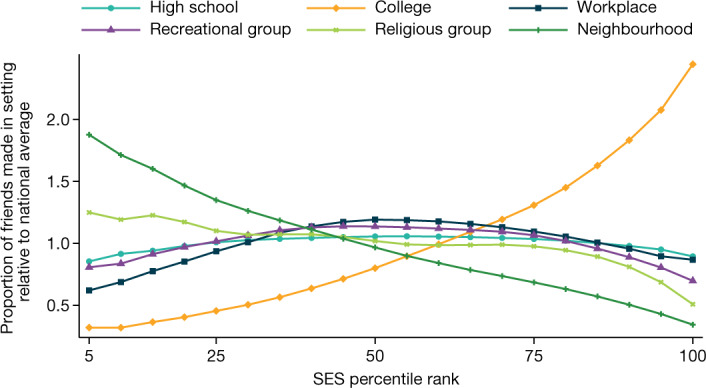
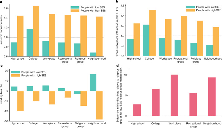
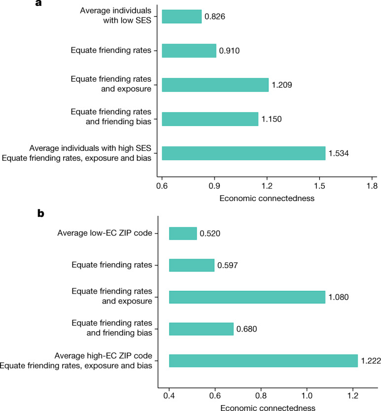
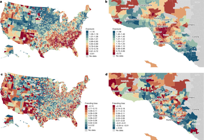
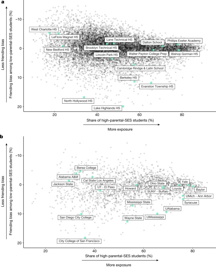
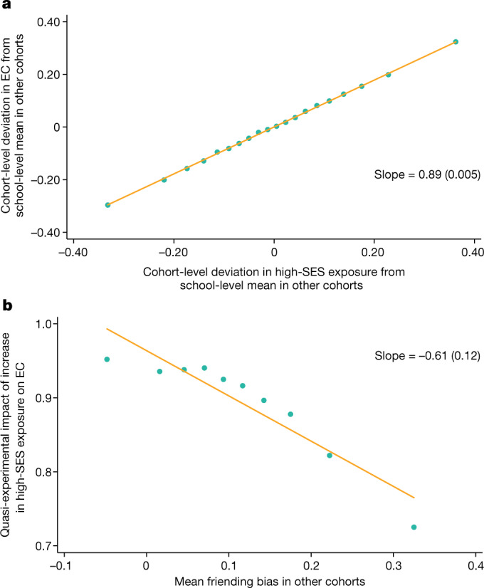
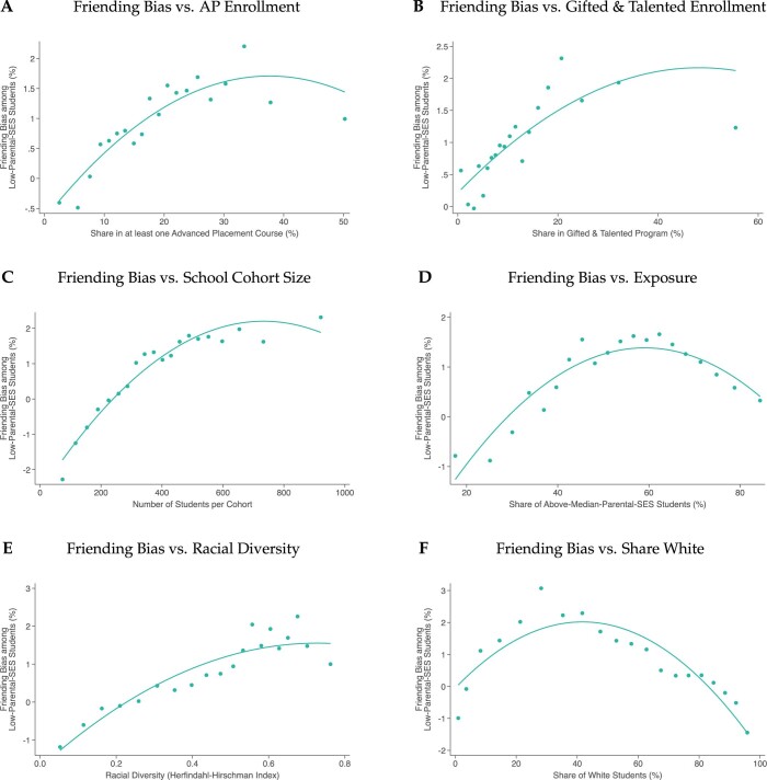
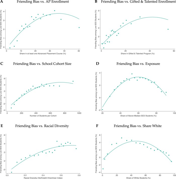
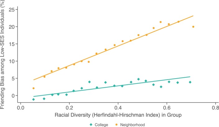
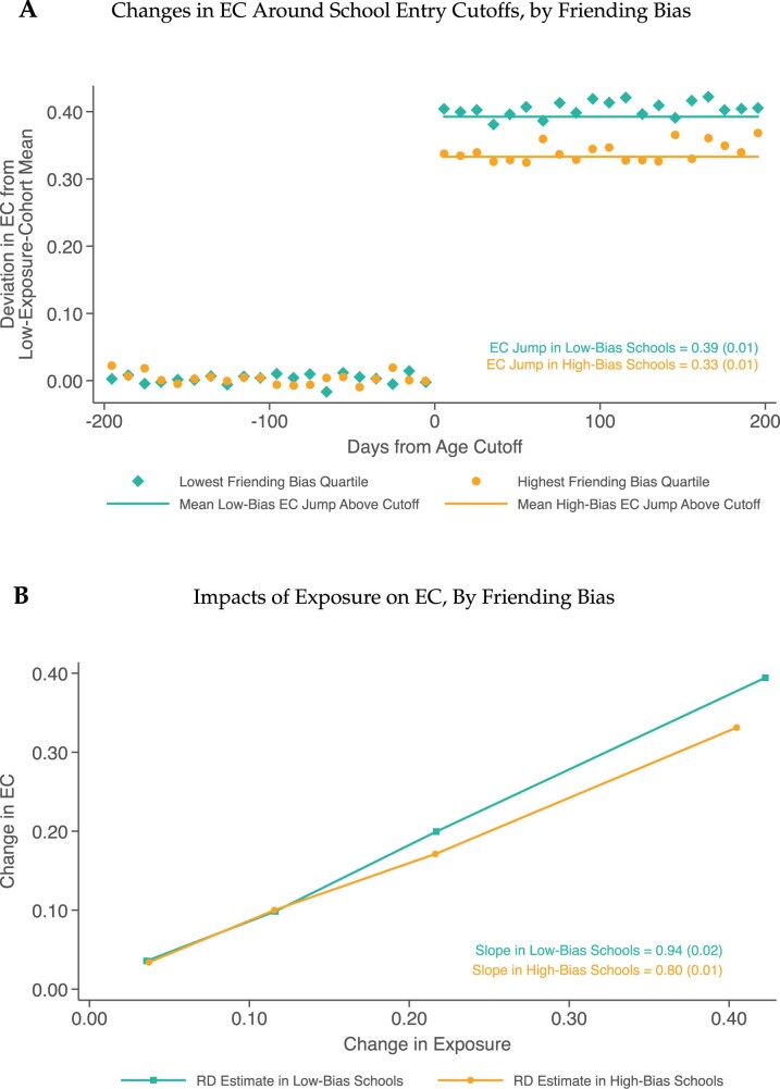
Low levels of social interaction across class lines have generated widespread concern^1-4 and are associated with worse outcomes, such as lower rates of upward income mobility^4-7. Here we analyse the determinants of cross-class interaction using data from Facebook, building on the analysis in our companion paper⁷. We show that about half of the social disconnection across socioeconomic lines-measured as the difference in the share of high-socioeconomic status (SES) friends between people with low and high SES-is explained by differences in exposure to people with high SES in groups such as schools and religious organizations. The other half is explained by friending bias-the tendency for people with low SES to befriend people with high SES at lower rates even conditional on exposure. Friending bias is shaped by the structure of the groups in which people interact. For example, friending bias is higher in larger and more diverse groups and lower in religious organizations than in schools and workplaces. Distinguishing exposure from friending bias is helpful for identifying interventions to increase cross-SES friendships (economic connectedness). Using fluctuations in the share of students with high SES across high school cohorts, we show that increases in high-SES exposure lead low-SES people to form more friendships with high-SES people in schools that exhibit low levels of friending bias. Thus, socioeconomic integration can increase economic connectedness in communities in which friending bias is low. By contrast, when friending bias is high, increasing cross-SES interactions among existing members may be necessary to increase economic connectedness. To support such efforts, we release privacy-protected statistics on economic connectedness, exposure and friending bias for each ZIP (postal) code, high school and college in the United States at https://www.socialcapital.org .

Fig. 1. Friending rates by setting and SES.

Friending rates across settings by the SES percentile rank of individuals in our primary analysis sample. The primary analysis sample consists of individuals between the ages of 25 and 44 years as of 28 May 2022 who reside in the United States, have been active on the Facebook platform at least once in the previous 30 days, have at least 100 US-based Facebook friends, have a non-missing residential ZIP code and for whom we are able to allocate at least one friend to a setting using the algorithm described in the ‘Variable definitions’ section of Methods. The vertical axis shows the relative share of friends made in each of the six settings that we analyse (for example, high schools), defined as the average fraction of friends made in that setting by people in a given SES ventile (5 percentile rank bin) divided by the fraction of friends made in that setting in the whole sample. Numbers above 1 imply that people at a given SES rank make more friends in a given setting than the average person; numbers below 1 imply the opposite. Extended Data Table 4 lists the underlying shares of friendships made in each setting for people with below-median SES versus above-median SES.

Fig. 2. EC, exposure and friending bias by setting and SES.

a–d, Variation in EC, exposure and friending bias across six settings where friendships are formed by individuals’ SES. All of the plots are based on the primary analysis sample defined in the legend of Fig. 1. a, Economic connectedness (EC) by setting for individuals with below-median SES (left, green bars) and above-median SES (right, orange bars). For both low- and high-SES individuals, EC is defined as twice the fraction of above-median-SES friends made within each setting. b, Mean rate of exposure to high-SES individuals in an individual’s group (for example, their high school) by setting for individuals with below-median SES (left, green bars) and above-median SES (right, orange bars). High-SES exposure is defined as two times the fraction of above-median-SES members of the individual’s group. c, Mean friending bias by setting for individuals with below-median SES (left, green bars) and above-median SES (right, orange bars). Friending bias is defined as one minus the ratio of the share of above-median-SES friends to the share of above-median-SES peers in the individual’s group. EC, high-SES exposure and friending bias are all calculated at the individual level and then aggregated to the setting × SES level (Supplementary Information B.5). d, Restricting the sample to low-SES members of religious groups, plots these individuals’ friending bias in each of the other settings minus their friending bias in religious groups. Extended Data Table 4 lists the values of average EC, bias and exposure shown in this figure.

Fig. 3. Determinants of differences in EC by SES and across ZIP codes.

a, Share of the difference in EC between individuals with high versus low SES that is driven by differences in the settings in which they make friendships (friending rates), rates of exposure to individuals with high SES in those settings and friending bias conditional on exposure. The first and fifth bars show the observed EC for average low- and high-SES individuals, calculated as the EC for individuals who have setting-level friending rates, exposure rates and friending bias levels that match the means for low- and high-SES people in our sample, respectively (Methods: ‘Decomposing EC’). The middle three bars show the predicted EC for the average low-SES individual under various counterfactual scenarios. In the second bar, we consider a counterfactual scenario in which the friending rates across different settings for the average low-SES individual are equated to those of the average high-SES individual, while preserving exposure and friending bias at the mean observed levels for low-SES individuals within those settings. The third bar further equates the rate of high-SES exposure in each setting to match the observed mean values for high-SES individuals. The fourth bar equates rates of friending bias in each setting as well as friending rates across settings to match the observed mean values for high-SES individuals. The fifth bar equates rates of both exposure and friending bias within settings and friending rates across settings. b, A decomposition exercise analogous to a between ZIP codes with different levels of EC for below-median-SES residents instead of between individuals with below- versus above-median SES. The comparison of interest here is between ZIP codes in the bottom quintile of the EC distribution for below-median-SES residents (low-EC ZIP codes) and ZIP codes in the top quintile of EC for below-median-SES residents (high-EC ZIP codes). See Supplementary Information B.5 for further details on these counterfactual exercises.

Fig. 4. The geography of exposure and friending bias.

a–d, Maps of mean high-SES exposure (a,b) and mean friending bias (c,d) for individuals with low SES. a,c, National county-level maps. b,d, ZIP-code-level maps of the Los Angeles metropolitan area. We aggregate individual-level statistics to compute ZIP-code-level and county-level means (Supplementary Information B.5). At the individual level, exposure is defined as the weighted average of two times the fraction of individuals with above-median SES in the groups in which an individual with below-median SES participates, weighting each group by the individual’s share of friends in that group. Friending bias is defined as one minus the weighted average of the ratio of the share of high-SES friends to the share of high-SES peers in the groups in which an individual with low SES participates, again weighting each group by the individual’s share of friends in that group. We use methods from the differential privacy literature to add noise to the statistics plotted here to protect privacy while maintaining a high level of statistical reliability; see www.socialcapital.org for further details on these procedures.

Fig. 5. Friending bias and exposure by high school and college.

a,b, Mean friending bias among students with low parental SES versus the share of students with high parental SES by high school (a) and college (b). Friending bias is defined as one minus the mean ratio of the share of high-school friends with high parental SES to the share of high-school peers with high parental SES, averaging over students with low parental SES (Supplementary Information B.5).The vertical axis is reversed, so that schools and colleges in the upper half of each panel have lower friending bias. The sample consists of individuals in the 1990–2000 birth cohorts (approximately spanning the high school and college graduating classes of 2008–2018 and 2012–2022, respectively) who could be linked to a specific school or college and to parents with an SES prediction. We report statistics only for high schools and colleges that have at least 100 low-SES and 100 high-SES Facebook users summing across these cohorts. We use methods from the differential privacy literature to add noise to the statistics plotted here to protect privacy while maintaining a high level of statistical reliability; see https://www.socialcapital.org for further details on these procedures. In this figure, SES refers to the SES of the individuals’ parents; Supplementary Fig. 2 replicates these figures using individuals' own (post-high school and post-college) SES ranks in adulthood.

Fig. 6. Cross-cohort estimates of the causal effects of socioeconomic integration on EC in high schools.

a,b, Analysis of the causal effect of being assigned to a high school cohort with more high-SES peers on the EC of low-SES students, based on the level of friending bias in the school (Methods: ‘Cross-cohort estimates’). a, Cohort-level changes in economic connectedness of low-SES students versus changes in the share of high-SES students. b, Causal impacts of high-SES share on economic connectedness of low-SES students, by level of friending bias. We measure EC, exposure and bias in this figure based on parental SES. The sample consists of all of the individuals in our primary analysis sample who were born between 1990 and 2000 whom we can link to parents and match to high schools. We further limit the sample to schools with at least 500 students (pooling all cohorts), at least 100 bottom-quintile-SES students and at least 100 top-quintile-SES students. For each cohort, exposure is defined as five times the fraction of top-quintile-SES students. EC in a cohort is defined as five times the average share of top-quintile-SES friends among bottom-quintile-SES students. Friending bias is defined as the average among bottom-quintile-SES students of one minus the ratio of the share of friends with top-quintile SES to the share of peers with a top-quintile SES in their cohort. In a, a binned scatter plot is shown of the cohort-level deviations from school means in EC versus cohort-level deviations from school means in exposure. The cohort-level deviations are constructed as the mean for the relevant cohort c in a given school minus the mean for all other cohorts in the same school, weighting by the number of students with bottom-quintile SES in each cohort. The binned scatter plot is constructed by dividing the cohort-level deviations in exposure into 20 equally sized bins and plotting the mean deviation in EC versus the mean deviation in exposure within each bin. We also report a slope estimated using a linear regression, with standard error clustered by high school in parentheses. To construct the plot in b, we first divide school × cohort cells into deciles based on the mean level of friending bias for all other cohorts in the same school. We then estimate regressions analogous to that in a using the school × cohort cells in each of the ten deciles separately. Finally, we plot the slopes from the ten regressions against the mean level of friending bias (leaving out the focal cohort) in each decile.

Extended Data Fig. 1. Predictors of Friending Bias in High Schools Using Parental SES.

This figure shows school-level binned scatter plots of the average degree of friending bias (based on parental SES) among low-SES individuals versus various school-level characteristics: the share of students enroled in at least one Advanced Placement course (Panel A); the share of students enroled in a Gifted and Talented program (Panel B); total number of students per cohort (Panel C); the share of above-median-parental-SES students (Panel D); an index of racial diversity defined as $\left(1-{\mathrm{\Sigma }}_i{s}_i^2\right)$, where s_i is the fraction of race/ethnicity i (Black, white, Asian, Hispanic, Native American) in the school (Panel E); and the share of white students (Panel F). Friending bias is defined as one minus the mean ratio of the share of high-SES high school friends to the share of high-SES high school peers, averaging over low-SES students in the 1990-2000 birth cohorts (see Supplementary Information B.5). Shares of students enroled in at least one AP course and in a Gifted and Talented program are obtained from the 2015–2016 Civil Rights Data Collection (CRDC). School size and racial composition data are from the 2017–2018 National Center Education Statistics (NCES) data (see Supplementary Information A.2). The set of schools used in these plots is the same as in Fig.5, conditional on being present in the CRDC data. To construct the binned scatter plots, we divide the variable on the horizontal axis into ventiles (5 percentile point bins) and plot the mean of the vertical-axis variable against the mean of the horizontal-axis variable in each ventile. All binned scatter plots are weighted by the number of students in each high school as reported in the NCES data. As a visual guide to approximate the non-parametric relationships, the solid lines in each figure show lines of best fit from quadratic regressions estimated using OLS.

Extended Data Fig. 2. Predictors of Friending Bias in High Schools Using Own SES.

This figure replicates Extended Data Fig. 1 using own SES rank in adulthood instead of parental SES rank when measuring friending bias and when defining the share of above-median SES students in Panel D. See notes to Extended Data Fig. 1 for further details.

Extended Data Fig. 3. Friending Bias versus Racial Diversity.

This figure presents binned scatter plots of friending bias against racial diversity within colleges (green diamonds) and neighbourhoods (ZIP codes, orange circles). See notes to Extended Data Fig. 1 for details on construction of binned scatter plots. We define racial diversity as $\left(1-{\mathrm{\Sigma }}_i{s}_i^2\right)$, where s_i is the fraction of race/ethnicity i (Black, white, Asian, Hispanic, Native American). Friending bias is defined as the average among below-median-SES individuals in the group (i.e., college or neighbourhood) of one minus the ratio of the share of above-median-SES friends in each individual’s group to the share of above-median-SES peers in that group. For comparability, both series measure SES using own SES rank in adulthood and use data from the 1986–1996 birth cohorts. Racial shares for each college and ZIP code are obtained from the 2013 Integrated Post-Secondary Education Data System (IPEDS) and the 2018 American Community Survey (ACS), respectively.

Extended Data Fig. 4. Causal Effects of Socioeconomic Integration on Economic Connectedness in High Schools: Regression-Discontinuity Estimates.

This figure analyses the causal effects of being assigned to a high school cohort with more high-SES peers on economic connectedness (EC) using a regression discontinuity design, separately for schools with low versus high levels of friending bias (Methods: ‘Regression Discontinuity Estimates’). The sample consists of all individuals in our analysis sample born between 1990 and 2000 whom we can link to their parents and match to high schools. Panel A shows the reduced-form impacts of jumps in the share of high-SES students on EC, separately by the level of friending bias. To construct Panel A, we first calculate the absolute values of changes in the fraction of students with top-quintile-parental-SES ("high-SES”) across all consecutive high-school cohort pairs. We then restrict the sample to cohort pairs in the top quartile of this distribution of exposure changes, and order cohorts so that the cohort with the lower share of high-SES students is the first of the two cohorts. We define EC for a given student as five times the share of top-quintile-parental-SES friends in their cohort. We then calculate means of EC for all bottom-quintile-parental-SES ("low-SES") students in a cohort pair, pooling students by their age distance in days from the cohort age cutoff (subtracting the mean EC among low-SES students in the cohort). We do this separately for schools in the top and bottom quartile of the distribution of friending bias, calculated as the average friending bias of low-SES individuals in the same high school over all cohorts excluding the own and adjacent cohorts. We report regression discontinuity (RD) estimates (with standard errors in parentheses) of the jump in average EC at the cutoff estimated using a linear regression with a bandwidth of 200 days; the solid lines plot the magnitudes of these jumps (Methods: ‘Regression Discontinuity Estimates’). In Panel B, we plot RD estimates of the jump in EC (estimated as in Panel A) for each of the four quartiles of changes in exposure across cohorts against the mean change in (normalized) high-SES exposure in that exposure-jump quartile. We again plot these estimates separately for schools in the top and bottom quartile of leave-out friending bias.

Extended Data Fig. 5. Relationship Between Friends’ Socioeconomic Status and Own Socioeconomic Status.

This figure plots the mean socioeconomic status (SES) percentile rank of individuals’ friends against their own SES percentile rank. The series in green circles is calculated using the entire friendship network for each individual. The series in orange squares is constructed using each individual’s ten closest friends, based on the frequency of public interactions such as likes, tags, wall posts, and comments. The green and orange series are identical to those in Fig. 1 of Chetty et al.. The series in purple triangles replicates the series in green circles using the 30% of friendships that we are able to assign to a group, the primary analysis sample used in this paper. For each series, we report slopes estimated from a linear regression on the plotted points, with heteroskedasticity-robust standard errors in parentheses.

References

1. Fischer CS, Mattson G. Is America fragmenting? Ann. Rev. Sociol. 2009;35:435–455. doi: 10.1146/annurev-soc-070308-115909. - DOI
1. Smith JA, McPherson M, Smith-Lovin L. Social distance in the United States: sex, race, religion, age, and education homophily among confidants, 1985 to 2004. Am. Sociol. Rev. 2014;79:432–456. doi: 10.1177/0003122414531776. - DOI
1. Doob, C. B. Social Inequality and Social Stratification in US Society (Routledge, 2019).
1. Putnam, R. D. Our Kids: The American Dream in Crisis (Simon and Schuster, 2016).
1. Alesina A, Baqir R, Easterly W. Public goods and ethnic divisions. Q. J. Econ. 1999;114:1243–1284. doi: 10.1162/003355399556269. - DOI