Distance decay 2.0 - A global synthesis of taxonomic and functional turnover in ecological communities

Abstract

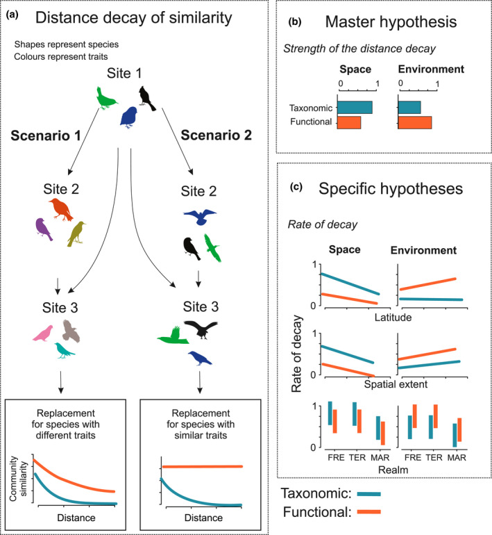
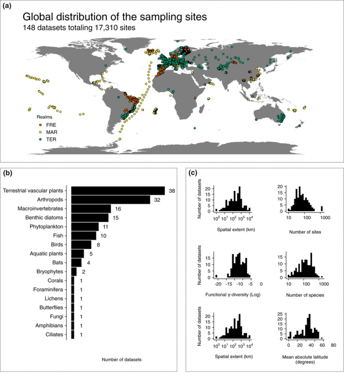
Aim: Understanding the variation in community composition and species abundances (i.e., β-diversity) is at the heart of community ecology. A common approach to examine β-diversity is to evaluate directional variation in community composition by measuring the decay in the similarity among pairs of communities along spatial or environmental distance. We provide the first global synthesis of taxonomic and functional distance decay along spatial and environmental distance by analysing 148 datasets comprising different types of organisms and environments.

Location: Global.

Time period: 1990 to present.

Major taxa studied: From diatoms to mammals.

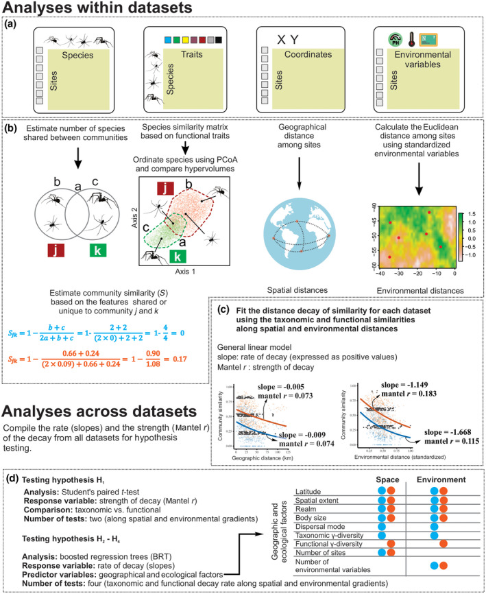
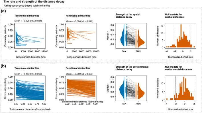
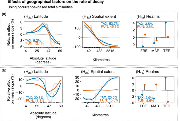
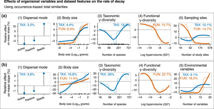
Method: We measured the strength of the decay using ranked Mantel tests (Mantel r) and the rate of distance decay as the slope of an exponential fit using generalized linear models. We used null models to test whether functional similarity decays faster or slower than expected given the taxonomic decay along the spatial and environmental distance. We also unveiled the factors driving the rate of decay across the datasets, including latitude, spatial extent, realm and organismal features.

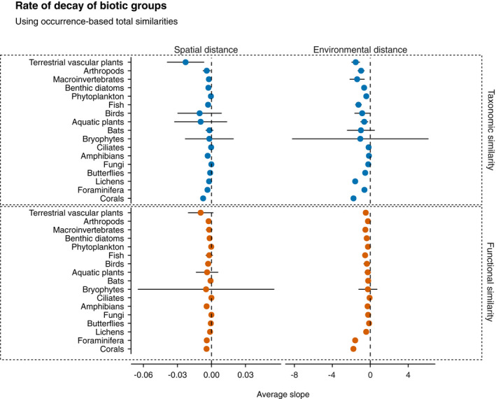
Results: Taxonomic distance decay was stronger than functional distance decay along both spatial and environmental distance. Functional distance decay was random given the taxonomic distance decay. The rate of taxonomic and functional spatial distance decay was fastest in the datasets from mid-latitudes. Overall, datasets covering larger spatial extents showed a lower rate of decay along spatial distance but a higher rate of decay along environmental distance. Marine ecosystems had the slowest rate of decay along environmental distances.

Main conclusions: In general, taxonomic distance decay is a useful tool for biogeographical research because it reflects dispersal-related factors in addition to species responses to climatic and environmental variables. Moreover, functional distance decay might be a cost-effective option for investigating community changes in heterogeneous environments.

Keywords: biogeography; environmental gradient; spatial distance; trait; β‐diversity.

FIGURE 1

(a) Taxonomic and functional distance decay. Two scenarios of distance decay of taxonomic and functional similarities along spatial and environmental distance. In scenario 1 (for simplicity, we consider here replacement only), the replacement occurs among species that have different traits (i.e., colours), which leads to both taxonomic and functional distance decay. In scenario 2, the replacement occurs among species that have similar traits, which leads to zero functional distance decay measured by the slope. (b) Master hypothesis: spatial distance decay is stronger for taxonomic similarities than for functional similarities, whereas environmental distance decay is stronger for functional similarities. (c) Specific hypotheses (higher values indicate steeper slopes) across datasets. For latitude, spatial distance decay is flatter in the datasets from higher latitude and, more notably, for taxonomic similarities than for functional similarities. Environmental distance decay is steeper in datasets from higher latitude for functional similarities, whereas it does not vary notably with latitude for taxonomic similarities. For spatial extent, both taxonomic and functional spatial distance decay are flatter in the datasets covering a larger spatial extent, whereas environmental distance decay is steeper in datasets covering a larger extent. For realm, marine ecosystems show flatter spatial and environmental distance decay than terrestrial and freshwater systems. Abbreviations: FRE = freshwater systems; MAR = marine systems; TER = terrestrial systems

FIGURE 2

Study design highlighting (a) a map of the study sites coloured according to the realms (FRE = freshwater; MAR = marine; TER = terrestrial); (b) the number of datasets for major biotic groups; and (c) the distribution of the datasets with respect to spatial extent, number of study sites, functional γ‐diversity (log₁₀ hypervolume SD³), taxonomic γ‐diversity (number of species), number of environmental variables and latitude

FIGURE 3

The analytical framework described in a stepwise manner: (a–c) hierarchical description of the methods performed at dataset level, including the estimation of similarities and distance in addition to the distance decay models of each dataset; and (d) description of the tests performed after the compilation of the metrics from all datasets. (a) The four objects used in the analyses: a species‐by‐traits table, a sites‐by‐species matrix, a sites‐by‐coordinates table and a sites‐by‐environment table. (b) The calculation of taxonomic and functional similarities and of spatial and environmental distance. In the first example, only species identities are considered, and because sites k and k do not share any species, community similarity (blue) equals zero. In the second example, the functional traits of species are considered, and community similarity (orange) is higher than zero. The third example shows how spatial distance was calculated as the geographical distance between pairs of sites using spatial coordinates. The fourth example illustrates how sites far from each other may show similar environmental conditions and therefore small environmental distance. Environmental distance was calculated as the Euclidean distance between pairs of sites considering the standardized environmental variables. (c) Illustration of the metrics extracted to study the distance decay across datasets. The strength of distance decay was measured from Mantel tests using Spearman correlations (Mantel r), and the rate of decay was measured as the slopes of generalized linear models following a quasibinomial family with a log link. The models were built separately for each response variable (taxonomic or functional similarity) and explanatory variables (spatial or environmental distance), totalling four Mantel r values and four slopes. Also, the data of marine fish from the Mediterranean Sea are shown as an example in which the distance decay of similarity along environmental distance is stronger (higher Mantel r) for functional similarity than for taxonomic similarity, irrespective of the rate of decay (slope). (d) Description of the analyses used to test the hypotheses and which metrics were considered for each analysis. The strength (Mantel r) of decay was used to test hypothesis H₁, and the rate of decay (slope) was used to hypotheses H₂–H₄

FIGURE 4

The distance decay along (a) spatial distance and (b) environmental distance. The light blue lines show the distance decay of taxonomic similarity, and the orange lines show the distance decay of functional similarity. The first and second columns show the rate (slope) of the taxonomic and functional distance decay, respectively; the third column shows the strength (Mantel r) of the distance decay of taxonomic and functional similarities; and the fourth column shows the standardized effect sizes of the slopes of each dataset

FIGURE 5

The average rate of decay (slopes) of biotic groups using occurrence data along spatial and environmental distance. The vertical dashed lines highlight the zero rate (absence of decay), and the horizontal lines indicate the standard deviation of the mean. The blue circles show the rate of decay of taxonomic similarities, and the orange circles show the rate of decay of functional similarities. Large error bars are attributable to low sample size (i.e., a low number of datasets for a given taxon)

FIGURE 6

Relative effects (expressed as percentages) of geographical factors on the rate of decay along (a) spatial distance decay and (b) environmental distance decay of the total component of taxonomic (TAX, light blue) and functional (FUN, orange) similarities using occurrence data across datasets. Partial dependence plots show the effects of a predictor variable on the response variable after accounting for the average effects of all other variables in the model. Positive values indicate an increase in the rate of decay (steeper slopes) compared with the mean rate, whereas negative values indicate a decrease in the rate of decay (flatter slopes) compared with the mean rate. Semi‐transparent lines represent the actual predicted effects; continuous lines represent LOESS fits to predicted values from boosted regression trees (BRTs). We show here only the variables related to the specific hypotheses [i.e., latitude, spatial extent and realms (FRE = freshwater; MAR = marine; TER = terrestrial)]

FIGURE 7

Relative effects (expressed as a percentage) of organismal variables and dataset features on the rate of decay along (a) spatial distance and (b) environmental distance, considering the total component of taxonomic (light blue lines) and functional (orange lines) similarities using occurrence data across datasets. Partial dependence plots show the effects of a predictor variable on the response variable after accounting for the average effects of all other variables in the model. Positive values indicate an increase in the rate of decay (steeper slopes) compared with the mean rate, whereas negative values indicate a decrease in the rate of decay (flatter slopes) compared with the mean rate. Semi‐transparent lines represent the actual predicted effects; continuous lines represent LOESS fits to predicted values from boosted regression trees (BRTs). We show here the organismal variables and the variables related to the dataset features

References

1. Anderson, M. J. , Crist, T. O. , Chase, J. M. , Vellend, M. , Inouye, B. D. , Freestone, A. L. , Sanders, N. J. , Cornell, H. V. , Comita, L. S. , Davies, K. F. , Harrison, S. P. , Kraft, N. J. B. , Stegen, J. C. , & Swenson, N. G. (2011). Navigating the multiple meanings of β diversity: A roadmap for the practicing ecologist. Ecology Letters, 14, 19–28. 10.1111/j.1461-0248.2010.01552.x - DOI - PubMed
1. Astorga, A. , Oksanen, J. , Luoto, M. , Soininen, J. , Virtanen, R. , & Muotka, T. (2012). Distance decay of similarity in freshwater communities: Do macro‐ and microorganisms follow the same rules? Global Ecology and Biogeography, 21, 365–375. 10.1111/j.1466-8238.2011.00681.x - DOI
1. Bagaria, G. , Pino, J. , Rodà, F. , & Guardiola, M. (2012). Species traits weakly involved in plant responses to landscape properties in Mediterranean grasslands. Journal of Vegetation Science, 23, 432–442. 10.1111/j.1654-1103.2011.01363.x - DOI
1. Barbaro, L. , Brockerhoff, E. G. , Giffard, B. , & van Halder, I. (2012). Edge and area effects on avian assemblages and insectivory in fragmented native forests. Landscape Ecology, 27, 1451–1463. 10.1007/s10980-012-9800-x - DOI
1. Barbaro, L. , Rusch, A. , Muiruri, E. W. , Gravellier, B. , Thiery, D. , & Castagneyrol, B. (2017). Avian pest control in vineyards is driven by interactions between bird functional diversity and landscape heterogeneity. Journal of Applied Ecology, 54, 500–508. 10.1111/1365-2664.12740 - DOI
LinkOut - more resources