A numerical population density technique for N-dimensional neuron models

Abstract

Population density techniques can be used to simulate the behavior of a population of neurons which adhere to a common underlying neuron model. They have previously been used for analyzing models of orientation tuning and decision making tasks. They produce a fully deterministic solution to neural simulations which often involve a non-deterministic or noise component. Until now, numerical population density techniques have been limited to only one- and two-dimensional models. For the first time, we demonstrate a method to take an N-dimensional underlying neuron model and simulate the behavior of a population. The technique enables so-called graceful degradation of the dynamics allowing a balance between accuracy and simulation speed while maintaining important behavioral features such as rate curves and bifurcations. It is an extension of the numerical population density technique implemented in the MIIND software framework that simulates networks of populations of neurons. Here, we describe the extension to N dimensions and simulate populations of leaky integrate-and-fire neurons with excitatory and inhibitory synaptic conductances then demonstrate the effect of degrading the accuracy on the solution. We also simulate two separate populations in an E-I configuration to demonstrate the technique's ability to capture complex behaviors of interacting populations. Finally, we simulate a population of four-dimensional Hodgkin-Huxley neurons under the influence of noise. Though the MIIND software has been used only for neural modeling up to this point, the technique can be used to simulate the behavior of a population of agents adhering to any system of ordinary differential equations under the influence of shot noise. MIIND has been modified to render a visualization of any three of an N-dimensional state space of a population which encourages fast model prototyping and debugging and could prove a useful educational tool for understanding dynamical systems.

Keywords: Python; dynamical systems; network; neural population; population density; simulator; software; visualization.

Figure 1

(A) The mesh used in MIIND to simulate a population of Izhikevich neurons. The quadratic red curve and blue line are the nullclines where the rate of change of the membrane potential and recovery variable, respectively, are zero. The strips, made up of quadrilateral cells are formed by the characteristic curves of the Izhikevich model for a given parameter set. (B) A vector field for the same model showing the direction of movement of probability mass around the state space. (C) The state space discretized into a regular grid. The parameters and definition of the Izhikevich model are not given here as it is only required to demonstrate the mesh and grid discretization. As in the original derivation of the model, the recovery variable has no units.

Figure 2

Figure showing steps for generating the transition matrix to solve the deterministic dynamics of the underlying model using a two-dimensional grid. Axes are not labeled as they represent arbitrary time-dependent variables. (A) For each grid cell (rectangle), the vertices translated according to a single time step of the underlying neuron model and the resulting quadrilateral is triangulated. (B) Each triangle is then tested for intersection with the axis-aligned lines of the original grid. The green crosses mark the intersection points between the tested triangle and the dashed line. The resulting subsections are again triangulated. (C) The process runs recursively until no more triangulations can be made. (D) The resulting triangles each lie within only a single cell of the original grid. The area of each triangle divided by the area of the original quadrilateral gives a proportion of mass to be transferred from the grid cell to the containing cell. From these, the proportions to be transferred can be summed and the totals stored in the file.

Figure 3

(A) The change in state, J, of a neuron due to a single incoming spike can be split into component parts, Jx and Jy for the horizontal and vertical dimensions, respectively. All neurons with a state within cell 0 will be translated by Jx due to a single incoming spike. Because all cells are the same width (Cx), the uniformly distributed probability mass of cell 0 will be shared among a maximum of two cells, cell 1 and cell 2. The offset of cell 1 from cell 0 is equal to floor(Jx/Cx) [for negative Jx, it is ceil(Jx/Cx)] with cell 2 being the one beyond that. The proportion of mass transferred from cell 0 to cell 1 is equal to 1 − (Cx%Jx) and the remainder is transferred to cell 2. (B) Once the mass proportions have been calculated in the horizontal direction, the same calculations are made with cells 1 and 2 in the vertical direction using Cy and Jy. The proportion calculated from cell 0 to cell 1 is split between cells 3 and 4. The proportion in cell 2 goes to 5 and 6. (C) The proportions of mass to be transferred from cell 0 to the resulting four cells give an approximation of the effect of transition J. With a constant J, this calculation gives the same relative results for every cell and therefore only needs to be performed once. (D) Iteratively applying the transitions to all cells in the grid spreads mass further across state space simulating the effect of neurons receiving multiple spikes in a given time step. (E) The probability mass function of a population of leaky integrate-and-fire neurons with an excitatory synaptic conductance rendered in MIIND. The color of each cell indicates the amount of probability mass. The value has been normalized to the maximum value of all cells. The effect of an incoming spike is to shift mass 0.2 nS/cm² in the vertical direction (producing a change in synaptic conductance). At this early point in the simulation, most neurons would have received zero or one spike (indicated by the bright yellow spots) while only a few would have received up to four spikes. (F) As the simulation proceeds, mass continues to be transferred upwards due to incoming spikes but the deterministic dynamics of the model causes mass to also move to the right according to the transitions defined in the matrix file and the population becomes more cohesive.

Figure 4

(A) With a three-dimensional state space, the grid discretization is made up of cuboids. (B) For the two-dimensional case, a rectangle has two possible triangulations, [A,B,C] and [A,C,D] or [A,B,D] and [B,D,C]. (C) A cuboid triangulated into six 3-simplices. Other triangulations are possible, some which aim to achieve the minimum number of simplices or to keep the volumes of the simplices as uniform as possible. The Delaunay triangulation makes no guarantees of this kind but is easy to implement and works in N-dimensions.

Figure 5

(A,D,G,J) Possible plane intersections with a 3-simplex. (B,E,H,K) Illustration of how each intersection is represented in the algorithm such that intersections bisect the relevant edges. (C,F,I,L) The resulting triangulations of the bisected 3-simplex which can be applied to all intersections of this type when calculating the transitions. (A–C) A plane intersection leaving one vertex of the 3-simplex above the plane and three vertices below. (D–F) A plane intersection leaving two vertices on either side of the plane. (G–I) A plane intersection which goes through one of the vertices leaving one vertex above the plane and two vertices below. (J–L) A plane intersection which goes through two vertices leaving one vertex on either side.

Figure 6

(A) A schematic of the E-I population network. The excitatory population, E is made up of N_E neurons. The inhibitory population, I contains N_I = 10, 000−N_E neurons. Each population receives an excitatory external input of 500 Hz. Each neuron in both populations receives 0.01N_E excitatory connections and 0.01N_I inhibitory connections. Arrows represent an excitatory connection, circles represent an inhibitory connection. (B) The three-dimensional state space of the leaky integrate-and-fire neuron with an excitatory and inhibitory synaptic conductance. v is the membrane potential, w is the excitatory synaptic conductance, and u is the inhibitory synaptic conductance. The vector field shows the direction of motion in state space for neurons with no external impulse. Neurons which receive an excitatory input spike are shifted higher in w. Neurons which receive an inhibitory input spike are shifted higher in u. The solid curves show trajectories of neurons under excitatory impulse alone. The dashed curves show trajectories of neurons under inhibitory impulse alone.

Figure 7

Visualizations of a population of leaky integrate-and-fire neurons with an excitatory and inhibitory synaptic conductance in MIIND. Cells with no probability mass are transparent. With increasing probability mass, they become more opaque and change from red to yellow. The color and opacity are normalized to the value of the cell with the highest probability mass. (A,C,E) The probability mass function across a 150 × 150 × 150 grid. (B,D,F) The probability mass function across a 50 × 50 × 50 grid for the same simulation time as the image above. (A,B) When the population receives only excitatory incoming spikes, the probability mass function remains in the plane at u = 0. (C,D) When the population receives only inhibitory incoming spikes, the probability mass function stays in the plane at w = 0. (E,F) When the population receives both inhibitory and excitatory incoming spikes, the probability mass function extends into the state space. In this case, the excitatory input is enough to overcome the inhibitory input and the mass function moves across the threshold potential. The bright face shows the probability mass at the threshold. Probability mass which has been reset reappears at the reset potential and moves further into the state space.

Figure 8

(A) The average membrane potential for a single population of leaky integrate-and-fire neurons with excitatory and inhibitory synaptic conductances simulated using a Monte Carlo approach and using MIIND with grids of different resolutions. (B) The effect on the average steady state membrane potential with different rates of the Poisson distributed input for the Monte Carlo simulation and different MIIND grid resolutions. (C) The effect on the average steady state excitatory conductance variable with increasing Poisson input rate. Only the mean of the values for the Monte Carlo simulation are shown here (without a variance or standard deviation) because the MIIND simulation produces no such statistic and so no comparison can be made.

Figure 9

(A) The average firing rate of a single population of leaky integrate-and-fire neurons with excitatory and inhibitory synaptic conductances simulated using a Monte Carlo approach and using MIIND with grids of different resolutions. (B) The effect on the average steady state firing rate of the population with increasing rate of the Poisson distributed input.

Figure 10

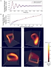
(A) The average membrane potential of the excitatory population in the E-I network with a ratio of 1:1 excitatory and inhibitory neurons (N_E = N_I). In the MIIND simulation, each connection between populations has the “number of connections” value set to 50. (B) The average membrane potential of the excitatory population in the E-I network with a ratio of 8:2 excitatory to inhibitory neurons (N_E = 8, 000, N_I = 2, 000). In the MIIND simulation, the excitatory connections have the “number of connections” value set to 80 and the inhibitory connections have the “number of connections” value set to 20. For clarity, the traces from the Monte Carlo simulation and the MIIND simulation have been separated. (C–H) The probability mass function for the excitatory population in MIIND during the double peaked oscillation with a connection ratio of 8:2. (H) shows the corresponding points in the oscillation. At (C), The population only experiences the external input of 500 Hz and is pushed toward the threshold. At (D), though some probability mass has passed threshold and been reset, the majority is close to the threshold and so the average membrane potential is at a peak. At (E), probability mass has continued to cross the threshold so that now a large amount is near the reset potential which brings the average back down. The function has also shifted higher in w due to the excitatory self-connections and more probability mass is pushed across threshold. The function also begins moving upwards in u from the increased inhibitory input but this is not enough to overcome the excitation. At (F), the inhibitory input has continued to push the probability mass function higher in u and much less probability mass now crosses the threshold. At (G), the function continues to shift back away from threshold approaching (C) once again.

Figure 11

(A) The average membrane potential of a single population of Hodgkin-Huxley neurons simulated using a Monte Carlo approach and in MIIND with a 50 × 50 × 50 × 50 grid. (B) The average steady state membrane potential with different rates of the Poisson distributed input. (C–E) The three-dimensional marginal probability mass function of the four-dimensional Hodgkin-Huxley neuron population in MIIND having reached a steady state. The membrane potential v, sodium activation variable m, and potassium activation variable n are shown. (F) The three-dimensional marginal probability mass function showing the gating variables, w, n, and h (sodium inactivation variable) only.

References

1. Barber C. B., Dobkin D. P., Huhdanpaa H. (1996). The quickhull algorithm for convex hulls. ACM Trans. Math. Softw. 22, 469–483. 10.1145/235815.235821 - DOI - PubMed
1. Bogacz R., Brown E., Moehlis J., Holmes P., Cohen J. D. (2006). The physics of optimal decision making: a formal analysis of models of performance in two-alternative forced-choice tasks. Psychol. Rev. 113, 700. 10.1037/0033-295X.113.4.700 - DOI - PubMed
1. Booth V., Rinzel J. (1995). A minimal, compartmental model for a dendritic origin of bistability of motoneuron firing patterns. J. Comput. Neurosci. 2, 299–312. 10.1007/BF00961442 - DOI - PubMed
1. Brette R., Gerstner W. (2005). Adaptive exponential integrate-and-fire model as an effective description of neuronal activity. J. Neurophysiol. 94, 3637–3642. 10.1152/jn.00686.2005 - DOI - PubMed
1. Brown K. Q. (1979). Voronoi diagrams from convex hulls. Inform. Process. Lett. 9, 223–228. 10.1016/0020-0190(79)90074-7 - DOI - PubMed
LinkOut - more resources